边缘智能

边缘学习范式

边缘智能

目的

为什么智能必须在其运行环境中自适应，而不能从遥远的训练中冻结下来？

在数据中心训练出的模型，部署到用户设备后会遇到新的条件。词汇、光照、声学以及使用模式可能与其参数所依据的分布不同，并且这一差距会随行为演化而扩大。集中式训练无法预见每一种上下文，也无法为每位用户个性化。原始观测数据也未必能够传输，因为存在隐私约束、带宽限制或延迟要求。设备端学习将自适应带到数据产生的位置。用 C³ 术语来说，计算转移到设备上，通信从原始观测缩减为选择性更新，协同则在边缘的功耗与内存预算内运行。

Learning Objectives

通过比较集中式云训练、设备端学习与联邦学习的数据流、隐私特性与运行权衡，形成对比
在内存、计算和能耗方面，量化边缘设备训练相对仅推理部署的开销
从能耗、热余量和前台延迟余量中推导后台自适应的准入条件
通过比较内存占用、表达能力与收敛性，针对特定设备能力选择模型自适应策略
应用数据效率技术（少样本学习、经验回放、对比学习），在数据有限的本地数据上学习而不产生灾难性遗忘
设计联邦学习系统，在聚合保护隐私的更新的同时，管理异构数据、通信效率与慢节点
说明设备端学习所需的运行控制：设备感知的部署、分布式验证、保护隐私的监控，以及面向异构人群的回滚

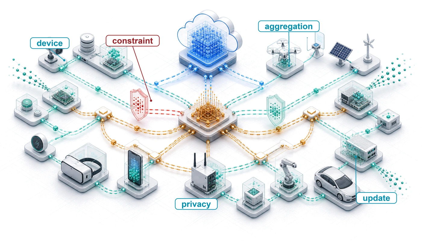
设想一个在云端数据中心基于数百万份通用音频样本训练出的语音助手。部署后，它可能难以应对地方口音或家庭专用词汇；若无本地自适应，其性能会随使用方式偏离训练分布而下降。边缘智能 将推理、自适应与协同置于观测数据的设备之上或附近，使模型能够在功耗、内存、隐私和连接性约束下响应本地上下文。

数据中心机器学习系统假定处于受控环境：计算资源充裕、网络连接可靠、系统行为可预测。集中式推理正是这一假设最典型的体现，而边缘则打破了它。

学习预测用户文本输入的智能手机、适应家庭日常习惯的智能家庭设备，以及依据本地驾驶条件更新感知模型的自动驾驶车辆，都展示了传统集中式训练方法力所不及的场景。智能手机会遇到个体用户独有的语言模式，而这些模式并不存在于全球训练数据中；智能家庭设备必须适应因家庭而异的季节变化与家庭动态；自动驾驶车辆则面临与原始训练环境不同的本地路况、天气模式与交通行为。

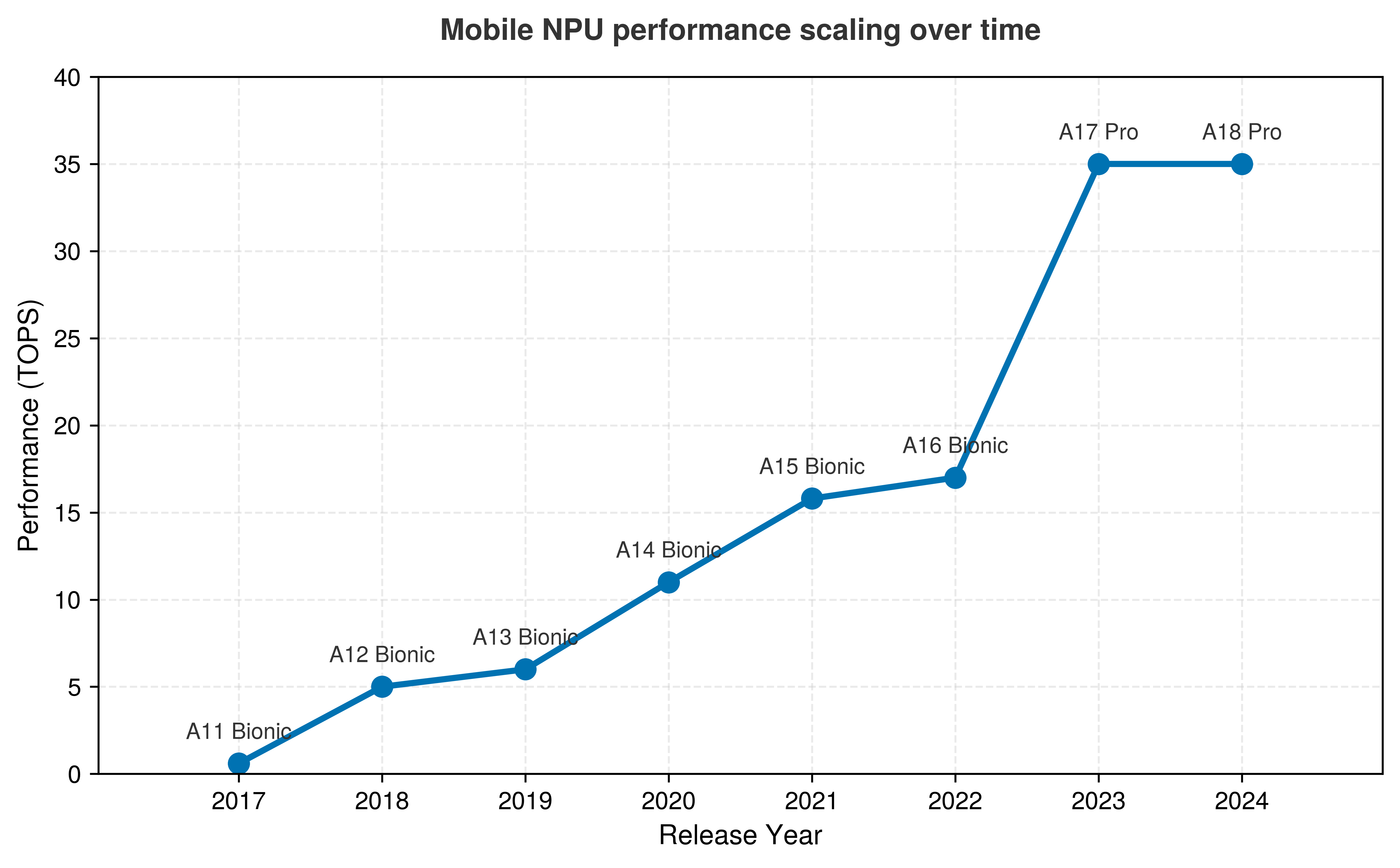
这些场景需要设备端学习，即模型在其运行所在设备上直接训练与自适应。¹ 机器学习由此从集中式训练转向跨越异构设备的分布式学习，每个设备都在本地约束下运行。在集群栈中，这使计算逼近设备的功耗、内存与热容量极限。使设备端自适应成为可行的，并非算法的改变，而是芯片的改变：移动加速器吞吐量在 移动 NPU 性能扩展 中绘制的曲线七年内增长了一个数量级以上，从而将训练型负载纳入手机的功耗包络。

¹ A11 Bionic（2017） ：苹果首款专用神经引擎的系统级芯片（SoC），面向机器学习推理负载的运算速率最高达每秒 6000 亿次。其系统层面的影响是确立了移动 NPU 为独立的功耗域：当面向推理优化的芯片为短时本地训练或个性化释放热余量后，设备端自适应便更具可行性。

:::

:::

本地适配只能发生在已经越过推理门槛的硬件上，因为一次梯度更新所付出的成本严格高于它所基于的前向传播。专用加速器设定了这一门槛：它们决定边缘设备是否具备足够的延迟与能量余量来运行智能工作负载，进而决定本地训练是否可能实现。

Systems Perspective 1.1: 专用 NPU 的硅基红利

在通用移动 CPU 与专用 NPU 之间运行同一模型，其差距最好被理解为一种”硅基红利”，而非边际加速。已发布的 NPU 性能档案会因硅代次和工作负载而异，因此本笔记本采用显式场景假设，而非直接报告基准测试：相对于所建模的 MobileNetV2 基线（20× 延迟改善、60× 能效改善，1.883 ms 每次推理）。这些乘数用于说明对加速器增益的敏感性；它们并非该具名移动档案或某特定 NPU 的实测属性。

对系统设计而言，重要的是这些比值所代表的差异类型。在上述假设下，专用硬件带来了可观的延迟与能量余量。该余量究竟使工作负载可行、允许持续后台执行，还是使 CPU 回退方案不可接受，必须借助针对工作负载与设备特定的延迟、功耗和热特性测量来确立。

向设备侧学习的转变，在机器学习系统设计层面引入了根本性的张力。基于云端的架构拥有充裕的计算资源与受控的运行环境，而边缘设备必须在极为受限的资源包络内运行。内存以兆字节而非吉字节计量；功耗预算以毫瓦而非瓦计量；网络连接可能间歇性中断，甚至完全不存在。当本地模型运行于安全关键回路时，这些约束便转化为生命安全工程问题。

这些约束贯穿 Archetype C（Federated MobileNet）（原型 C（联邦 MobileNet）），其中自主性要求学习必须在严苛的资源限制下于设备上完成。Archetype C 代表了这一谱系中的极端一端。在毫瓦级功耗预算下，它无法承担将原始数据上传至云端的能量成本。因此，数据本地性是由功耗墙所强加的物理必然，而不仅仅是一项隐私特性。量化训练、稀疏更新与联邦协同，是使 Archetype C 得以存在的生存策略。

要驾驭这一架构张力，需要沿用推理领域的压缩技术，并结合使极端资源约束下有效学习成为可能的算法技术、设计模式与系统原则。这一挑战超出了对训练算法的常规优化：它要求重新思考整个机器学习流水线，以适配传统计算假设失效的部署环境。

Definition 1.1: 设备侧学习

设备侧学习 指无需服务器连接，直接在部署硬件上对机器学习模型进行本地训练或适配。

重要性：它使超个性化与自主运行成为可能，而严苛的资源约束下。在铁律的框架内，设备侧学习必须最小化每次更新所消耗的总能量，因为每个梯度步都依赖有限的电池电量，并与系统中的其他任务争夺可用的计算吞吐量 $(R_{\text{peak}})$。
区别：与仅执行固定模型的 Edge Inference 不同，设备侧学习涉及一个本地优化回路（前向与反向传播），需要显著更多的内存与计算资源。
常见误区：一种常见误解是，设备侧学习需要从零开始训练。实际上，它几乎总是 On-Device Adaptation：微调一个预训练基础模型的小部分参数，以适配本地环境的具体数据分布。

其影响已超出技术优化，延伸至机器学习生命周期的每个阶段。模型从可预测的版本管理范式转变为持续的演化与自适应轨迹。性能评估从集中式监控仪表盘转向面向异构用户群体的分布式评估。隐私保护成为塑造系统设计决策的核心架构性要求，而非下游的合规性事项。

动机与收益

机器学习系统传统上依赖集中式训练流水线。大规模分布式基础设施允许模型在集中管理的数据集上开发和完善 (Dean 等 2012年)。训练完成后，这些模型可部署到客户端设备用于推理，从而形成训练与部署阶段之间的清晰分离。尽管这种架构分离在许多应用场景中表现良好，但在本地数据具有动态性、私密性或高度个性化特征的应用中，它也带来了显著局限。

Dean, Jeffrey, Greg Corrado, Rajat Monga, Kai Chen, Matthieu Devin, Quoc V. Le, Mark Z. Mao, 等. 2012年. 《Large Scale Distributed Deep Networks》. 收入 Advances in Neural Information Processing Systems (NeurIPS), 编辑 Peter L. Bartlett, Fernando C. N. Pereira, Christopher J. C. Burges, Léon Bottou, 和 Kilian Q. Weinberger, 卷 25. Curran Associates.

² 隐私保护（差分隐私）：联邦学习虽然避免了原始数据的移动，但研究表明原始梯度可以被”反演”以重构输入样本。差分隐私通过加入经过校准的噪声，将任何一条记录或用户在给定邻域定义下所贡献的隐私损失加以约束；它能够降低推理风险，但保证的强度取决于 $\varepsilon$、$\delta$、组合方式与实现质量。

设备侧学习通过使系统能够在设备上直接训练或适配、而不依赖对云端的持续连接，挑战了这一既定模式。这一转变反映了不断变化的应用需求与用户期望，后者要求具备响应迅速、个性化且隐私保护²的机器学习系统。

边缘侧学习先撞上内存墙，而非算力墙。

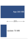
考虑一款智能手机输入法，它需要适应用户独特的词汇量和打字习惯。为了个性化预测，系统必须使用本地观察到的文本输入，对紧凑的语言模型执行梯度更新。即使是最小的语言模型，单次梯度更新也需要 50 MB–100 MB 的内存用于激活和优化器状态。智能手机操作系统通常只给输入法等后台应用留下 200 MB–300 MB 的内存，具体预算会因操作系统、设备代次和前台负载而有所不同。这极窄的余量凸显了边缘侧学习所面临的核心工程挑战：单个训练步骤就可能消耗 25 percent 的可用内存。系统必须在如此严苛的约束下实现有意义的个性化，而传统训练方法在架构上已不可行。这一量化现实推动了对专门技术的需求，使资源极度受限条件下的自适应成为可能。

四项关键考量推动了从集中式学习向分布式学习的转变 (Li 等 2020年)：个性化、延迟与可用性、隐私，以及基础设施效率。个性化是最具吸引力的动机，因为已部署的模型常常会遇到与训练环境不同的使用模式和数据分布。本地自适应使模型能够针对用户特定数据优化行为，捕捉语言偏好、生理基线、传感器特性或环境条件。这种能力在高用户间差异的应用中至关重要，因为单一全局模型无法有效服务所有用户。

延迟与可用性约束为本地学习提供了进一步的正当性。在边缘计算场景中，与集中式基础设施的连接可能不可靠、延迟，或出于节省带宽、降低能耗而被有意限制。边缘侧学习使模型能够在完全离线或对延迟敏感的场景中自主改进，而往返云端的更新在架构上不可行。

隐私考量构成了第三项有力驱动因素。许多应用涉及敏感或受监管数据，包括生物测量、输入文本、位置轨迹或健康信息。本地学习可以通过将原始数据保留在设备上、并将传输到集中式系统的数据量降至最低来降低隐私暴露。这可以简化合规工程，但它本身并不能确立对《通用数据保护条例》(GDPR)³、《健康保险可携性与问责法案》(HIPAA)⁴ (U.S. Department of Health and Human Services 2026年) 以及特定区域数据主权法律的遵守。

³ GDPR（通用数据保护条例）: 自 2018 年 5 月起生效，GDPR 要求个人数据处理具备合法基础、数据最小化、目的限制以及权利处理流程。敏感场景下可能需要明示同意，但同意并非唯一的合法基础。边缘侧学习可以减少传输到集中式系统的个人数据量，并简化部分跨境和留存问题，但部署仍需具备与数据和用例相匹配的同意、权利和治理机制。

⁴ HIPAA（健康保险可携性与问责法案）: 要求受覆盖主体和业务伙伴对受保护健康信息（PHI）实施管理、物理和技术保障措施。代表受覆盖主体或业务伙伴创建、接收、维护或传输电子 PHI 的云服务，通常需要有适当的业务伙伴协议和安全规则控制。边缘侧学习可以减少 PHI 传输和供应商管理风险，但并不免除范围内医疗部署的 HIPAA 义务。

U.S. Department of Health and Human Services. 2026年. The HIPAA Security Rule. HHS.gov guidance.

基础设施效率为分布式学习方法提供了经济动机。集中式训练流水线需要大量后端基础设施来收集、存储和处理来自潜在数百万台设备的数据。将学习转移到边缘可以降低通信成本，并将训练工作负载分散到部署集群中，从而缓解对集中式资源的压力并提升可扩展性。

替代方案与决策标准

边缘智能：设备端学习

设备端学习需要可观的工程投入，而这种投入未必总是合理的。更简单的替代方案往往能以更低的运行开销达到相当的结果，而过早采用只会引入复杂性，却没有相应的价值。

设备端学习的替代方案 比较了三类替代方案，它们通常能在无需本地训练复杂性的情况下满足个性化与自适应需求。

**设备端学习的替代方案**：更简单的个性化机制可以在无需本地梯度更新的情况下满足许多自适应需求，因此设备端学习应仅保留在隐私、延迟、连接性或可测量的质量要求排除了这些选项的场景中。
替代方案	机制	何时适用
基于特征的个性化	将用户偏好、交互历史和行为特征保存在本地，然后将这些特征输入静态模型，而不是调整模型权重。	新闻推荐系统可以本地保存主题偏好和阅读习惯，再将这些特征与集中式内容模型结合。
带隐私控制的云端微调	将自适应集中到云端，在业务低峰时段以隐私保护技术（如差分隐私、联邦分析、安全聚合(Bonawitz 等 2017年)，或这些控制的组合）批量处理用户数据。	该方法通常比资源受限的设备端更新获得更高的准确率，同时为许多应用保持了可接受的隐私特性。
用户专属查找表	通过维护一个轻量级表格来保存频繁访问的本地模式，将全局模型与个性化检索机制结合起来。	当个性化收益明显，而计算和存储开销都很低时适用。

⁵ 差分隐私：一种通过向计算结果加入校准后的噪声来限制信息泄露的数学框架。在边缘学习中，这种噪声会转化为系统成本，因为更嘈杂的更新通常需要更多轮次或更多数据才能达到相同的效用。安全与隐私 阐述了正式的隐私预算机制。

在云端微调这一行中，差分隐私⁵ 是限制信息泄露的机制，但它所加入的噪声可能需要更多轮次或更多数据。

是否实施设备端学习，应当由可量化的需求驱动，而这些需求排除了上述更简单的替代方案。以下属于设备端学习采用的合法驱动因素：在法律上禁止云端处理的真实数据隐私约束、无法保证可靠连接的真正网络限制、排除云端往返的定量延迟预算，以及能够证明性能提升、从而证明运行复杂性的价值。

对于具有严格时延要求的应用，网络往返时间使得云端替代方案在架构上不可行。相机处理低于 33 ms、语音响应低于 500 ms、AR/VR 从运动到光子的延迟低于 20 ms，或安全关键控制低于 10 ms，这些场景所面临的网络往返时间通常在 50 到 200 ms 之间。在此类场景中，无论复杂性如何，设备端学习都是必需的。团队应在承诺设备端学习所需的重大工程投入之前，充分评估更简单的解决方案。

以知识迁移作为自适应基础

这些动机源于更广泛的知识迁移概念，即预训练模型将有用的表示迁移到新任务或新领域。这一基础性原则使得设备端学习既可行又有效，能够以极少的本地资源实现精细的自适应。图 1 展示了知识如何在密切相关任务（如玩不同的棋类游戏或乐器）之间发生迁移，也展示了如何在共享结构的领域之间发生迁移，例如从骑自行车到骑滑板车。在设备端学习中，一个在云端预训练的模型仅使用本地数据和有限的更新就能高效地适应新上下文，即使新任务在输入模态或目标上有所差异，也能实现快速自适应，而无需从头重新学习。

图 1: 知识迁移：预训练模型通过复用已有表示来加速新任务上的学习，例如在相关棋类游戏或乐器之间迁移技能。这种迁移还跨越领域，例如骑自行车与骑滑板车，共享的底层结构使得在有限的新数据下也能高效适应。

这一概念转变，借助迁移学习与自适应得以实现，使现实世界中的端侧应用成为可能。无论是为个人打字偏好适配语言模型、针对个体动作模式调整手势识别，还是在不断变化的环境中重新标定传感器模型，端侧学习都使系统能够随时间推移持续保持响应性、高效性与用户一致性。

现实应用领域

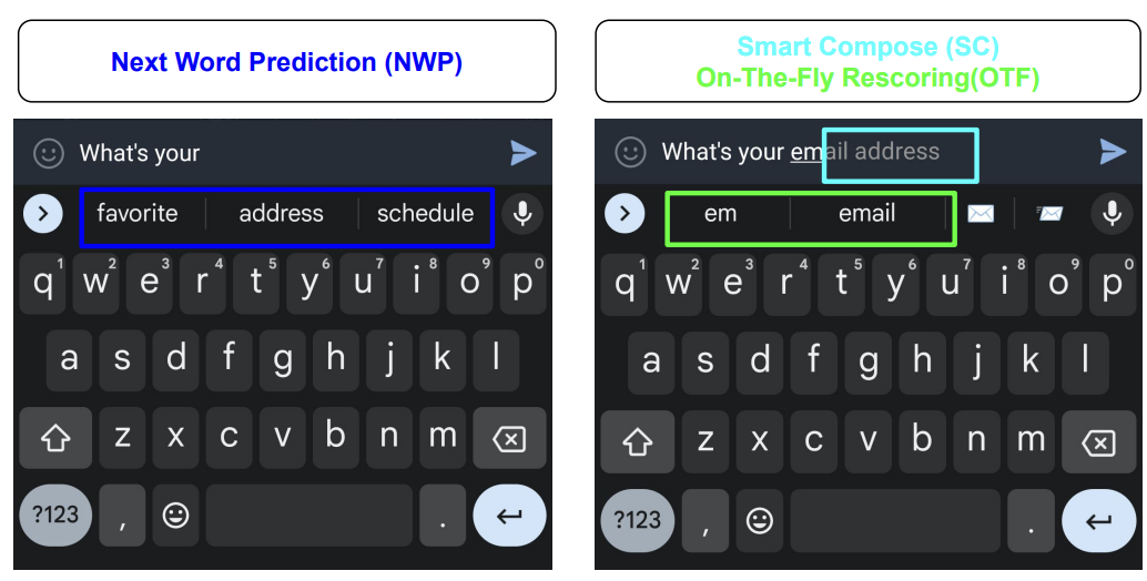
端侧学习的动机在消费技术、医疗、工业系统和嵌入式应用中具体呈现，每个领域都提供了使个性化、延迟、隐私和基础设施效率成为关键要求的场景。移动输入预测是端侧学习的一个有据可查的实例。在智能手机键盘等系统中，预测文本和自动更正功能能够从持续的本地自适应中显著受益。用户打字模式具有高度个性化特征并动态演化，因此集中式静态模型无法为高质量的用户体验提供足够支持。端侧学习使语言模型能够在设备上直接微调其预测，在实现个性化的同时保持数据本地性。Google 的 Gboard⁶ 例如，采用联邦学习来改进覆盖大量用户的共享模型，同时使原始数据保留在各设备本地(Hard 等 2018年)。

⁶ Gboard（2017）：这是最早被广泛报道的、在移动规模上部署的商用联邦学习方案之一。已发表的报告显示，键盘模型能够从聚合的端侧更新中获益，而原始输入文本仍保留在设备本地。其系统层面的影响是持久的：压缩后的更新与隐私机制使得在受限的移动网络上进行跨集群学习成为可能，而无需将原始按键数据集中。

Hard, Andrew, Kanishka Rao, Rajiv Mathews, Swaroop Ramaswamy, Françoise Beaufays, Sean Augenstein, Hubert Eichner, Chloé Kiddon, 和 Daniel Ramage. 2018年. 《Federated Learning for Mobile Keyboard Prediction》. arXiv preprint arXiv:1811.03604.

图 2展示了两种推理阶段的预测策略。下一个词预测根据当前上下文推测可能的续写内容，而 Smart Compose 则通过即时重打分提供动态补全。这些机制通过本地上下文个性化即时交互；更长周期的模型改进则通过联邦训练单独完成，聚合符合条件的端侧更新。

图 2: **端侧预测策略**：Gboard 在推理阶段于本地执行下一个词预测和 Smart Compose 重打分。这些请求时刻的机制利用本地上下文，而无需将每次按键发送到中央服务器；异步联邦训练则是单独的过程，用于从符合条件的端侧更新中改进共享模型参数。

可穿戴与健康监测设备提供了同样具有吸引力的应用场景，并附带额外的监管约束。这些系统依赖加速度计、心率传感器和皮肤电活动监测器提供的实时数据，以跟踪用户健康与体能状况。个体之间的生理基线差异显著，形成了静态模型无法有效应对的个性化挑战。端侧学习使模型能够随时间适应这些个体基线，在满足数据本地化监管要求的同时，显著提升活动识别、压力检测和睡眠分期的准确性。

语音交互技术是另一个重要的应用领域，具有独特的声学挑战。智能音箱和耳机等设备中的唤醒词检测⁷与语音界面，必须在嘈杂或动态变化的声学环境中快速、准确地识别语音指令。

⁷ 唤醒词检测：常开式关键词检测通常运行在亚毫瓦到低毫瓦的功耗范围内，远低于完整语音识别的功耗，采用针对亚 100 ms 延迟和极低误触发率优化的紧凑神经网络。这一极端的功耗约束定义了设计空间：模型必须足够小，以便在专用的常开处理器上运行，从而在不增加模型规模的前提下，使端侧个性化对于降低误触发率至关重要。

这些系统面临严格的延迟要求。语音界面必须将端到端响应时间控制在 500 ms 以内，以维持自然的对话流程，而唤醒词检测则需要亚 100 ms 的响应时间，以避免用户挫败感。本地训练使模型能够适应用户独特的语音特征与不断变化的环境上下文，从而降低误报率和漏检率，同时满足这些严苛的性能约束。这种自适应能力在远场音频场景中尤为有价值，因为不同部署的麦克风配置和房间声学条件差异显著。

除了消费类应用，工业物联网与远程监测系统展示了端侧学习在资源受限环境中的价值。在农业感知、管道监测或环境监控等应用中，与集中式基础设施的连接可能受限、昂贵，甚至完全不可用。端侧学习使这些系统能够在无需与云端持续通信的情况下检测异常、调整阈值或适应季节性趋势。这种能力对于维持边缘部署传感器网络的自主性与可靠性是必要的，因为系统停机或漏检可能带来显著的经济或安全后果。

最具挑战性的应用出现在嵌入式计算机视觉系统中，包括机器人、AR/VR 和智能摄像头。这些系统将复杂的视觉处理与节 1.0.2 中确立的最严格的延迟预算相结合：30 FPS 摄像头的 33 ms 帧预算、防止 AR/VR 眩晕的低于 20 ms 的运动到光子延迟预算，以及安全关键控制的低于 10 ms 的延迟上限。这些系统还运行在新颖或快速变化的环境中，这些环境与其原始训练条件存在显著差异。设备端自适应 使模型能够针对新的光照条件、物体外观或运动模式重新校准，同时满足这些关键的延迟预算；这些预算从根本上决定了采用设备端处理还是云端处理的架构选择。

每个领域都呈现出一种共同模式。部署环境引入了集中式训练期间无法预见的变化和特定情境下的需求。这些应用展示了推动设备端学习的动因如何体现为具体的工程约束。移动设备键盘在存储用户特有模式时面临内存限制。可穿戴设备受到能量预算的约束，训练频率因而受限。语音接口必须满足低于 100 ms 的延迟要求，因而无法采用云端协同。工业物联网系统运行在网络受限的环境中，要求具备自主适应能力。这一模式揭示了塑造后续所有技术决策的根本设计要求。学习必须在显著的资源约束下高效、保护隐私且可靠地进行。节 1.1 系统地分析这些约束，节 1.2 介绍在严格的资源限制内调整模型的技术，节 1.4 则确立设备群体之间保护隐私的协同协议。

架构权衡：集中式与去中心化训练

这些应用表明，设备端学习不仅改变了部署目标，也改变了训练生命周期。在集中式系统中，模型在数据中心基于汇总的数据集进行训练，以静态制品的形式部署到客户端，并通过离线重新训练获得定期更新。这种方法提供了充足的计算资源、多样化的数据以及成熟的调试和验证流程。它还假定数据传输可靠、集中托管数据可以接受，并且基础设施能够管理整个设备集群的更新—而边缘部署可能无法满足这些假设。

设备端学习颠覆了这些假设。每台设备维护自己的模型副本，并利用集中式基础设施无法获得的数据在本地进行自适应。训练以异步方式进行，其资源条件随设备使用模式、电池电量和热状态而变化。原始数据保留在设备上，降低了隐私暴露风险，但也增加了协同的复杂性。不同设备的硬件能力、运行环境和使用模式差异巨大，使学习过程具有异构性，难以标准化。

去中心化引入了一类新的系统挑战。设备可能运行不同的模型版本，导致整个部署设备集群的行为不一致。当客户端间歇性参与并在异构硬件上执行时，评估与验证会变得更加复杂 (Bonawitz 等 2019年)。必须谨慎管理模型更新，以防止性能退化；缺少集中式测试基础设施时，安全保证也更难落实。

管理数千台异构边缘设备的复杂性超出了典型分布式系统的水平。设备异构性不仅体现在硬件差异上，还包括不同的操作系统版本、安全补丁、网络配置和电源管理策略。大规模联邦系统必须能够容忍未通过资格检查、迟到或在训练轮次中退出的客户端 (Bonawitz 等 2019年)。还有一些设备已断开连接数周或数月，造成持续的协同挑战。

断开连接的设备重新连接时，需要进行状态协调以避免版本冲突。更新验证变得至关重要，因为设备可能未能应用更新却不报错，也可能报告更新成功，但仍运行过时的模型。鲁棒的系统采用多阶段验证。密码学签名确认更新的完整性，功能测试验证模型行为，遥测数据确认部署成功。回滚策略必须能够处理部分部署的情况，即一些设备已接收更新，而其他设备仍使用先前版本。在故障恢复期间维持系统一致性，需要复杂的编排机制；这些机制借鉴分布式系统原理，同时还需应对边缘环境特有的复杂性。

尽管存在这些挑战，去中心化仍能在无需集中监管的情况下实现深度个性化，支持在断开连接或带宽受限的环境中学习，并降低模型更新的运营成本。核心问题是如何协调设备之间的学习，而这一问题贯穿三个运行阶段：集中式训练、本地自适应和联邦协同。

边缘智能

传统集中式范式始于聚合数据上的云端训练，随后将静态模型部署到客户端设备。当数据采集可行、网络连接可靠，且单一全局模型能有效服务所有用户时，这种方法表现良好。然而，当数据变得个性化、涉及隐私敏感，或采集于连接受限的环境中时，该方法便难以为继。

部署之后，随着每台设备各自遇到独特的数据分布，本地差异逐渐显现。设备收集的数据反映了个体用户模式、环境条件和 usage 场景。此类数据往往是非独立同分布（non-IID⁸）且带有噪声的，因此需要本地模型适配以维持性能。这一转变标志着从全局泛化到本地专业化的过渡。

⁸ 非独立同分布（Non-IID，即 Not Independent and Identically Distributed）: 样本并非取自单一共同分布的数据，这是联邦学习中每台设备反映单个用户模式的默认条件。非独立同分布的标签与特征分布会显著劣化联邦平均性能，相对于独立同分布（i.i.d.）基线 (Zhao 等 2018年)，迫使系统采用本地适配层或聚类聚合等技术以维持收敛。

Zhao, Yue, Meng Li, Liangzhen Lai, Naveen Suda, Damon Civin, 和 Vikas Chandra. 2018年. 《Federated Learning with Non-IID Data》. CoRR abs/1806.00582.

最后阶段引入联邦协同，设备通过聚合后的模型更新周期性同步各自的本地适配，而非共享原始数据。这使得在保持数据本地性的同时，实现保护隐私的全局优化，并保留本地个性化的收益。

图 3 追溯了这一演进过程：从集中式训练，到本地适配，再到联邦协同。每个阶段都提高了协同复杂度，同时带来了纯集中式部署无法实现的能力。

边缘智能：训练开销

图 3: 从仅本地学习（区域 A）到集中式云端训练（区域 B），再到联邦协同（区域 C），代表了机器学习架构的根本性转变。每个阶段都引入了不同的运行特征，从孤立的本地模型，到统一的全球模型，再到协同的分布式学习。

去中心化、持续的学习重新定义了系统设计规则。系统不再运行于恒温恒湿的数据中心、拥有近乎无限的电力；它必须直面边缘设备严峻的物理与算法限制。

设计约束

在智能手机上微调神经网络受到功耗与散热的约束。GPU 训练集群可能消耗兆瓦级功率，而智能手机必须在约 10 W 的热预算内完成反向传播。在持续 10 W 的功耗下，理想化的 15 Wh 电池大约 1.5 小时即耗尽，而热不适感或降频可能更早地限制工作负载。因此，设备端学习必须精打细用地使用计算、内存与数据。

关于参数、运算与数据的约束是相乘而非相加地相互作用，由此形成的受约束优化问题远比仅部署推理要困难得多。最重要的转变在于压缩的目的。量化减少了每个权重的字节数，剪枝去除了不必要的参数，知识蒸馏将行为迁移到更小的架构中，而设备端学习则把这些工具从可选优化变成了基线可行性要求。这里确立的压缩基线，正是后续各节所依托的基础，而非需要重新推导的内容。

设备端学习遵循与推理相同的效率约束，但叠加了训练特有的放大效应，使得优化困难得多。推理只需对网络执行一次前向传播，而训练则需要前向传播、通过反向传播计算梯度，以及权重更新，在纳入激活值、梯度和优化器状态后，内存需求增加 4–12$\times$ 倍，计算开销增加 2–3$\times$ 倍。这些放大效应正是压缩基线在边缘不可妥协的原因：没有它，在这些设备约束下完成训练将不可能实现。

塑造设备端学习实现的根本工程挑战，直接源于上述动机。要在设备上启用学习，就必须彻底重新思考关于机器学习系统在哪里、如何运行的传统假设。在集中式环境中，模型训练可以依托庞大的计算基础设施、规模可观且经过筛选的数据集，以及充裕的内存与能源预算。而在边缘，这些假设无一成立，从而形成了一个根本不同的设计空间。

这些约束界定的是一个可行域，而非一份检查清单。模型压缩决定了算法可以改变到什么程度；稀疏且非均匀的数据决定了每个本地更新能够提取多少信号；有限的计算能力决定了训练究竟能否运行。这些维度之间的相互作用，决定了后续在自适应、数据效率与联邦协同技术之间做出何种选择。

量化边缘设备上的训练开销

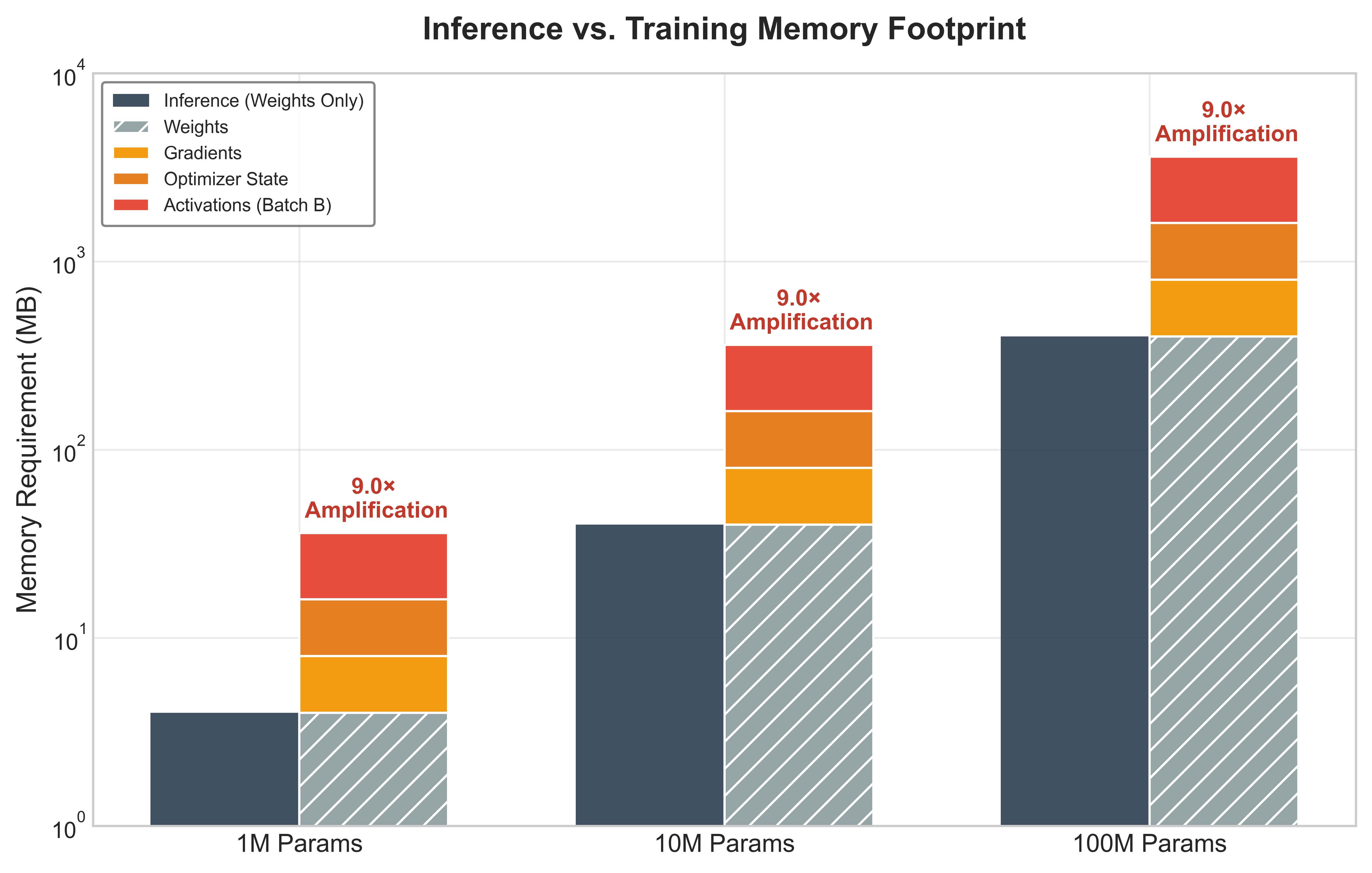
除压缩基线之外，训练以与本地自适应相关特有的方式放大了内存占用、内存带宽与硬件利用率方面的压力，且这些压力是相乘叠加而非简单相加。训练放大了推理约束 量化了计算运算如何增长 2–3$\times$ 倍、能耗如何飙升至 10–50$\times$ 倍，而图 4 则展示了该更宽区间内一个代表性的 9$\times$ Adaptive Moment Estimation（Adam）风格内存预算。

**训练放大了推理约束**：设备端学习遵循与推理相同的效率约束，但叠加了训练特有的放大效应，使优化困难程度显著增加。该表量化了从运行预训练模型切换到本地自适应时，每个约束维度如何被强化。放大系数假设采用标准反向传播，未采用梯度检查点等优化手段。
约束维度	推理	训练放大	对设计的影响
内存占用	模型权重 + 单张激活图	权重 + 完整激活缓存 + 梯度 + 优化器状态	增加 4–12$\times$ 倍；迫使激进压缩
计算运算	仅前向传播	前向 + 反向 + 权重更新	增加 2–3$\times$ 倍；限制模型复杂度
内存带宽	顺序读取权重	梯度双向数据流	增加 5–10$\times$ 倍；形成瓶颈
每样本能耗	单次推理操作	带收敛的多步梯度更新	增加 10–50$\times$ 倍；需要机会式调度
数据需求	预先采集、经过筛选的数据集	稀疏、含噪、流式本地数据	必须采用样本高效的方法
硬件利用率	针对前向传播优化	反向传播采用不同的访问模式	推理加速器可能无法帮助训练

一个代表性的 Adam 风格训练预算（图 4）在不同模型规模下可达到 9$\times$ 倍的内存占用增加；更宽的 4–12$\times$ 倍区间则取决于优化器选择、批大小、激活值检查点以及更新层数。

图 4: **训练内存放大器**：各柱状条比较 1M 至 100M 参数模型规模下的推理与训练内存。该示意配置存储权重、梯度、优化器状态与激活值，产生一个代表性的 9$\times$ 内存占用增加。

峰值内存使用量

训练期间的内存消耗并非一成不变。它会动态波动，在反向传播时达到峰值，因为此时激活值、梯度与优化器状态必须同时驻留。这一峰值内存决定了模型能否在某台设备上完成训练。例如，一个 10M 参数模型在配备 8 GB RAM 的智能手机上训练时，40 MB 的 FP32 权重可能在反向传播期间飙升至 200 MB 以上，因为激活值、梯度和优化器状态不断累积——与操作系统及前台应用直接争夺设备有限的内存。梯度检查点（gradient checkpointing）等技术通过这种方式缓解问题：在正向传播时丢弃中间激活值，并在反向传播时按需重新计算 (Chen 等 2016年)。这种做法以额外的计算量换取更低的峰值内存；具体节省多少，取决于检查点化了哪些激活值，以及设备能够容忍多少重计算。

这些放大效应解释了为何标准优化技术在不加修改的情况下应用于训练任务时会失效。每一类约束都会影响边缘侧学习系统的设计，因而需要采用在推理导向方法基础上构建、同时又加以扩展的方法。

Checkpoint 1.1: 边缘侧训练约束

验证对训练如何放大边缘侧约束的理解：

训练内存膨胀：解释为何同一模型在边缘侧训练通常比边缘侧推理需要多 4$\times$ 到 12$\times$ 倍的内存。
资源受限的 NPU：解释为何一个高速 NPU 仍可能闲置，因为训练流水线无法在设备的内存预算内持续供给数据与激活值。
反向传播 OOM：解释为何一个 10M 参数模型在配备 8 GB RAM 的智能手机上仍可能在反向传播期间触发内存不足（out-of-memory）错误。
检查点能耗：评估“梯度检查点可降低边缘侧训练总能耗”这一说法。

图 5 展示了完整的训练流水线如何在资源受限的物联网设备上，将离线预训练与在线自适应学习结合起来。系统首先使用通用数据进行元训练（meta-training）。部署阶段，设备特有的约束——数据可用性、计算能力和内存——通过排序和选择需要更新的层与通道来塑造自适应策略。这种选择性微调使得在有限的资源预算内实现高效的边缘侧学习成为可能。

\begin{tikzpicture}[line join=round,font=\sffamily\small]
\tikzset{
 Line/.style={line width=0.35pt,black!50,text=black,-latex},
 LineD/.style={line width=0.75pt,black!50,text=black,dashed,dash pattern=on 5pt off 3pt},
   Box/.style={inner xsep=2pt,
   node distance=0.45,
    draw=BlueLine,
    line width=0.75pt,
    fill=BlueL,
    minimum width=15mm, minimum height=7mm
  },
 circles/.pic={
\pgfkeys{/channel/.cd, #1}
\node[circle,draw=\channelcolor,line width=\Linewidth,fill=\channelcolor!10,
minimum size=6.5mm](\picname){};
        }
}
\pgfkeys{
  /channel/.cd,
  channelcolor/.store in=\channelcolor,
  drawchannelcolor/.store in=\drawchannelcolor,
  scalefac/.store in=\scalefac,
  Linewidth/.store in=\Linewidth,
  picname/.store in=\picname,
  channelcolor=BrownLine,
  drawchannelcolor=BrownLine,
  scalefac=1,
  Linewidth=0.6pt,
  picname=C
}

\begin{scope}[local bounding box=CIRCLE1,shift={($(0,0)+(0,0)$)},
scale=1, every node/.append style={transform shape}]
%1 column
\foreach \j in {1,2,3} {
  \pgfmathsetmacro{\y}{(1.5-\j)*0.83 + 0.7}
  \pic at (-1.35,\y) {circles={channelcolor=BrownLine,picname=1CD\j}};
}
%2 column
\foreach \i in {1,...,4} {
  \pgfmathsetmacro{\y}{(2-\i)*0.83+0.7}
  \pic at (0,\y) {circles={channelcolor=BrownLine, picname=2CD\i}};
}
%3 column
\foreach \j in {1,2} {
  \pgfmathsetmacro{\y}{(1-\j)*0.83 + 0.7}
  \pic at (1.35,\y) {circles={channelcolor=BrownLine,picname=3CD\j}};
}
\foreach \i in {1,2,3}{
  \foreach \j in {1,2,3,4}{
\draw[Line](1CD\i)--(2CD\j);
}}
\foreach \i in {1,2,3,4}{
  \foreach \j in {1,2}{
\draw[Line](2CD\i)--(3CD\j);
}}
\end{scope}

\begin{scope}[local bounding box=CIRCLE2,shift={($(CIRCLE1.east)+(4.0,-0.3)$)},
scale=1, every node/.append style={transform shape}]
%1 column
\foreach \j/\col in {1/RedLine,2/RedLine!40!,3/RedLine} {
  \pgfmathsetmacro{\y}{(1.5-\j)*0.83 + 0.7}
  \pic at (-1.35,\y) {circles={channelcolor=\col,picname=1CD\j}};
}
%2 column
\foreach \i/\col in {1/RedLine,2/BrownLine,3/BrownLine,4/RedLine!40!} {
  \pgfmathsetmacro{\y}{(2-\i)*0.83+0.7}
  \pic at (0,\y) {circles={channelcolor=\col, picname=2CD\i}};
}
%3 column
\foreach \j/\col in {1/RedLine,2/BrownLine} {
  \pgfmathsetmacro{\y}{(1-\j)*0.83 + 0.7}
  \pic at (1.35,\y) {circles={channelcolor=\col,picname=3CD\j}};
}
\foreach \i in {1,2,3}{
  \foreach \j in {1,2,3,4}{
\draw[Line](1CD\i)--(2CD\j);
}}
\foreach \i in {1,2,3,4}{
  \foreach \j in {1,2}{
\draw[Line](2CD\i)--(3CD\j);
}}
\end{scope}

\begin{scope}[local bounding box=CIRCLE3,shift={($(CIRCLE2.east)+(3.2,-0.3)$)},
scale=1, every node/.append style={transform shape}]
%1 column
\foreach \j/\col in {1/green!60!black!90!,2/green!60!black!90!,3/green!60!black!90!} {
  \pgfmathsetmacro{\y}{(1.5-\j)*0.83 + 0.7}
  \pic at (-1.35,\y) {circles={channelcolor=\col,picname=1CD\j}};
}
%2 column
\foreach \i/\col in {1/green!60!black!90!,2/BrownLine,3/BrownLine,4/green!60!black!90!} {
  \pgfmathsetmacro{\y}{(2-\i)*0.83+0.7}
  \pic at (0,\y) {circles={channelcolor=\col, picname=2CD\i}};
}
%3 column
\foreach \j/\col in {1/green!60!black!90!,2/BrownLine} {
  \pgfmathsetmacro{\y}{(1-\j)*0.83 + 0.7}
  \pic at (1.35,\y) {circles={channelcolor=\col,picname=3CD\j}};
}
\foreach \i in {1,2,3}{
  \foreach \j in {1,2,3,4}{
\draw[Line](1CD\i)--(2CD\j);
}}
\foreach \i in {1,2,3,4}{
  \foreach \j in {1,2}{
\draw[Line](2CD\i)--(3CD\j);
}}
\end{scope}
%\node[single arrow,fill=red!80!black!90, inner ysep=2pt,
    %  minimum width = 12pt, single arrow head extend=2pt,
      %minimum height=12mm] at($(CIRCLE2.east)!0.5!(CIRCLE3.west)$){};
\draw[brown!70,line width=6pt,shorten <=4pt,shorten >=4pt,
-{Triangle[width=1.8*6pt,length=0.9*6pt]}](CIRCLE2.east)
-- coordinate(SR1) (CIRCLE3.west);
\draw[brown!70,line width=6pt,shorten <=4pt,shorten >=4pt,
-{Triangle[width=1.8*6pt,length=0.9*6pt]}](CIRCLE1.east)
--coordinate(SR) (CIRCLE2.west);
\draw[brown!70,line width=6pt,shorten <=4pt,shorten >=4pt,
{Triangle[width=1.8*6pt,length=0.9*6pt]}-](CIRCLE1.west)
--node[above=6pt,align=center,text=black](PTB){Pre-trained\\ backbone}++(-2,0);

\begin{scope}[local bounding box=BOXX,shift={($(CIRCLE2.north)+(-1.1,1.5)$)}]
\node[Box](2B1)at(0,0){Data};
\node[Box,right=of 2B1](2B2){Compute};
\node[Box,right=of 2B2](2B3){Memory};
\node[draw=BackLine,inner xsep=3mm,line width=0.75pt,inner ysep=5mm,
fill=none,yshift=-2mm,fit=(2B1)(2B3)](BB){};
\node[below=1pt of BB.south,anchor=south]{Device Specific};
\end{scope}
\draw[brown!70,line width=6pt,shorten <=4pt,shorten >=4pt,
-{Triangle[width=1.8*6pt,length=0.9*6pt]}](BB.west)-|
    node[right=2pt,pos=0.85,text=black]{$s_i$}(SR);
\draw[brown!70,line width=6pt,shorten <=4pt,shorten >=4pt,
{Triangle[width=1.8*6pt,length=0.9*6pt]}-](SR1)--++(0,2);
%%
\node[below=4pt of CIRCLE1,align=center](T1){Meta-training with generic\\
     data (e.g., MiniImageNet)};
\node[below=4pt of CIRCLE2,align=center](T2){Rank the channels and layers based\\
     on the multi-objective metric $s_i$};
\node[below=4pt of CIRCLE3,align=center](T3){Train the selected\\ layers and channels};
%
\scoped[on background layer]
\node[LineD,draw=BrownLine,inner xsep=5mm,inner ysep=5mm,minimum height=74mm,
fill=BrownL!10,yshift=4mm,fit=(T2)(BB)(T3)](BB2){};
\node[below=1pt of BB2.north,anchor=north]{Online Adaptive Learning on IoT Devices};
\scoped[on background layer]
\node[LineD,draw=BackLine,inner xsep=3mm,inner ysep=5mm,
minimum height=74mm,
fill=yellow!05,yshift=14.7mm,fit=(T1)(PTB)(CIRCLE1)](BB2){};
\node[below=1pt of BB2.north,anchor=north]{Offline Pre-training};
\end{tikzpicture}

图 5: 资源受限设备采用两阶段学习流程。离线预训练确定初始模型权重；在线自适应则依据可用数据、计算能力和内存，选择性地更新各层。该方法在模型性能与边缘部署的实际限制之间取得平衡，从而支持真实环境中的持续学习。

模型约束

机器学习模型的结构与规模直接决定了设备端训练是否可行。部署于云端的模型可以包含数十亿个参数，并依赖数 GB 的内存预算；面向设备端学习的模型则必须满足对内存、存储和计算复杂度的严格约束。在训练过程中，这些约束进一步收紧，因为梯度计算、参数更新和优化器状态管理都需要推理之外的额外资源。

这些约束的程度在不同类型的设备上体现得十分具体。MobileNetV2 常用于移动端视觉任务，其标准配置需要约 14 MB 的存储空间。虽然这对拥有数 GB 可用 RAM 的智能手机而言是可行的，但却远远超出 Arduino Nano 33 BLE Sense 等微控制器所具备的 256 KB SRAM 和 1 MB 闪存容量。⁹ 在这类资源极其受限的平台上，即使单个卷积层，也可能因中间特征图和梯度的存储需求而在训练期间超出可用 RAM 容量。

⁹ Arduino Nano 33 BLE Sense: 其 SRAM 容量为 256 KB，约小 65,536×，比较基准是旗舰智能手机的 16 GB；单幅 $224{\times}224{\times}3$ RGB 图像占用 ~151 KB，消耗约 60 percent 的可用内存；激活值和梯度的存储还会增加若干需要同时驻留内存的张量，而优化器状态可能使训练的内存占用远超推理。这意味着，即使一个极小的卷积神经网络（CNN）层，也可能在反向传播期间超出 SRAM 总容量。这道内存墙迫使 8 位或 4 位量化成为先决条件，而非优化手段。

训练过程本身会大幅增加实际内存占用。标准反向传播在前向传播期间缓存各层的激活值，然后在反向传播的梯度计算中复用这些激活值。约束放大分析已经表明，与仅用于推理的部署相比，这种激活值缓存会使内存需求成倍增加。一个看似规模不大的 10 层卷积模型，在处理 $64{\times}64$ 图像时，可能需要 1 至 2 MB 内存，远超大多数嵌入式系统的 SRAM 容量。

模型复杂度还会直接影响运行时的能耗和热限制。在智能手表或电池供电的可穿戴设备中，持续训练模型可能迅速耗尽储备电量，或触发温控降频，导致性能下降。即使满足内存约束，从能耗角度来看，在这些设备上使用浮点运算训练完整模型也往往不可行。MLPerf Tiny 等超轻量基准为资源极其受限的设备提供了小型量化推理任务 (Banbury 等 2021年)。设备端自适应技术则通过冻结大部分参数、减少激活值存储或选择稀疏的更新参数集合来降低训练成本 (Cai 等 2020年; Kwon 等 2024年)。

Banbury, Colby, Vijay Janapa Reddi, Peter Torelli, Jeremy Holleman, Nat Jeffries, Csaba Kiraly, Pietro Montino, 等. 2021年. 《MLPerf Tiny Benchmark》. arXiv preprint.

电池与热约束的实际影响，并不仅限于限制训练时长。移动设备必须仔细权衡训练机会与用户体验。激进的端侧训练会导致明显的设备发热和快速耗电，进而引发用户不满，甚至导致应用被卸载。智能手机的机器学习工作负载通常运行在可持续处理包络 2–3 W 之内，以避免热不适；但在热节流触发前，它们可以短时突增到 5–10 W。即使训练规模不大的模型，也很容易超出这些可持续的功率上限。这一现实要求采用智能的调度策略：在充电期间进行训练以改善散热，在可能的情况下使用低功耗核心计算梯度，并实施感知温度的占空比控制，在温度超过阈值时暂停训练。一些系统甚至利用设备使用模式，仅在夜间充电、设备空闲且已接电时进行高强度的模型适配。

这些约束要求模型架构从一开始就针对端侧学习进行设计。大型 Transformer 和深度卷积网络若不进行切分、量化或卸载，根本无法用于端侧适配。专门的轻量架构，如 MobileNets¹⁰、SqueezeNet (Iandola 等 2016年) 和 EfficientNet (Tan 和 Le 2019年)，通过深度可分离卷积¹¹、瓶颈/火瓶模块以及复合模型缩放等机制，应对资源受限的推理。量化与选择性更新则是在架构之上叠加的独立部署与适配选择。

¹⁰ MobileNet (2017): Google 的架构借助深度可分离卷积，在标准 CNN 基础上实现了 8–9$\times$ 倍的 FLOPs 减少。系统层面的影响是：MobileNetV2 在 Pixel 手机上完成 ImageNet 分类约需 75 ms，而 ResNet-50 需要 1.8 秒，从而跨越了智能手机 2–3 W 功率包络内实时端侧推理与适配变得热可持续的门槛。

Iandola, Forrest N., Song Han, Matthew W. Moskewicz, Khalid Ashraf, William J. Dally, 和 Kurt Keutzer. 2016年. 《SqueezeNet: AlexNet-level accuracy with 50x fewer parameters and <0.5MB model size》. ArXiv preprint abs/1602.07360.

Tan, Mingxing, 和 Quoc V Le. 2019年. 《EfficientNet: Rethinking Model Scaling for Convolutional Neural Networks》. International Conference on Machine Learning (ICML), 6105～14.

¹¹ 深度可分离卷积: 将标准卷积分解为逐通道的深度可分离滤波器，随后进行 $1{\times}1$ 点积组合。对于一个 $3{\times}3$ 卷积（512 个输入/输出通道），参数量从 2.36 M 降至约 267 K，减少 8.8$\times$ 倍。这些收益是物理层面的，而非仅仅理论上的：正是这种分解使得移动 CPU 上实现实时 CNN 推理成为可能，同时也降低了端侧训练期间激活缓存所需的内存。

Howard, A. G., M. Zhu, B. Chen, D. Kalenichenko, W. Wang, T. Weyand, M. Andreetto, 和 H. Adam. 2017年. 《MobileNets: Efficient Convolutional Neural Networks for Mobile Vision Applications》. CoRR abs/1704.04861.

Sandler, Mark, Andrew Howard, Menglong Zhu, Andrey Zhmoginov, 和 Liang-Chieh Chen. 2018年. 《MobileNetV2: Inverted Residuals and Linear Bottlenecks》. 2018 IEEE/CVF Conference on Computer Vision and Pattern Recognition, 4510～20. https://doi.org/10.1109/cvpr.2018.00474.

模块化是一项关键的设计属性。MobileNets (Howard 等 2017年) 与 MobileNetV2 (Sandler 等 2018年) 可以通过不同的宽度倍率和分辨率设置进行配置，以在性能与资源占用之间取得平衡。一个完整的 MobileNetV2（宽度倍率 $\alpha_{\text{width}}=1.0$）约有 3.5M 个参数（14 MB 以 FP32 计）。在 $\alpha_{\text{width}}=0.5$ 条件下，完整的 1000 类模型约有 2.0M 个参数（7.9 MB），而仅含特征提取器、并带有一个小型任务特定头的部署，参数可少至 0.69M（2.8 MB），并可在 4 MB 的模型预算内完成。

数据约束

模型架构决定了端侧学习的内存与计算基线，但数据可得性与质量引入了同样根本性的限制，并影响学习过程的方方面面。端侧机器学习系统可获得的数据，与云端训练所用的大规模、经过精心策划的数据集相比，差异极大。在边缘侧，数据为本地采集，时间上稀疏，且往往非结构化或未标注。由此产生的数据量、质量与统计分布方面的挑战，直接影响了端侧学习的可靠性与泛化能力。

数据量受到存储约束与用户交互的间歇性双重严重限制。智能健身手环可能仅在身体活动时采集运动数据，因而每天产生的带标签样本相对较少。如果用户锻炼 30 分钟，可用于训练的数据点可能仅有几百个，而有效的监督学习通常需要数千甚至数百万个样本。这种稀缺性迫使算法从“数据丰富型”转向“数据高效型”。

端侧数据通常也非独立同分布（i.i.d.）(Zhao 等 2018年)，由此产生出云端系统很少遇到的统计挑战。部署到多个家庭的语音助手会面对口音、语言、说话风格与指令模式的广泛差异。智能手机键盘会依据个人打字模式、自动纠错偏好以及用户间差异显著的 multilingual 使用习惯进行自适应。这种异质性既使模型收敛更加困难，也增加了设计更新机制的难度——该机制必须能在不同设备之间实现泛化，同时保持个性化。

标签稀缺进一步加剧了数据分布问题。大多数在边缘端采集的数据默认没有标签，因而要求系统从弱监督或隐式监督信号中学习。智能手机摄像头可能在一天中拍摄数千张图像，但只有少数图像与有意义的用户操作（标记、收藏或分享）相关联，而这些操作可以充当隐式标签。在许多应用中，包括传感器数据的异常检测和手势识别的自适应，显式标签可能完全不可用；如果没有弱监督或无监督自适应的替代方法，传统监督学习便无法实施。

数据质量带来了进一步的挑战。环境传感器或汽车 ECU 等嵌入式系统会受到传感器校准波动、环境干扰或机械磨损的影响，导致输入信号随时间推移出现损坏或漂移。如果没有集中式验证系统来检测并过滤这些错误，它们就会在不易察觉的情况下降低学习性能。

隐私与安全方面的考量施加了最严格的约束，往往使数据共享在架构上无法实现，而不仅仅是不可取。根据法律和伦理要求，健康数据、个人通信或行为模式等敏感信息必须得到保护，防止未经授权的访问。因此，设备端学习必须依赖能够在始终不暴露敏感信息的前提下实现本地自适应的技术，从根本上重塑学习系统的设计与验证方式。

计算约束

边缘硬件为机器学习提供了计算基础，其范围涵盖资源最受限的 STM32F4 和 ESP32 等微控制器、中间层级配备专用 AI 加速器（Apple Neural Engine、Qualcomm Hexagon、Google Tensor）的移动级处理器，以及高端的高性能边缘设备。尽管这些设备提供了不同水平的推理能力（执行预训练模型时的计算吞吐量、内存带宽和能效），训练工作负载却呈现出根本不同的计算特征，从而重塑硬件的利用模式。

设备端学习必须在有限的计算能力范围内运行，而其原始计算能力与云端训练基础设施相比，相差数百倍甚至数千倍。关键差异在于：由于需要计算梯度和缓存激活值，反向传播所需的内存带宽显著高于推理；权重更新会产生写密集型访问模式，与推理的只读操作不同；优化器状态管理还需要分配额外的内存。完全足以支持推理的硬件，可能完全无法满足自适应的需求，即使只更新一小部分参数也是如此。

在资源最受限的一端，STM32F4¹² 或 ESP32¹³ 等微控制器仅提供几百 KB 的 SRAM，以及有限的计算和功耗预算 (Warden 和 Situnayake 2020年)。尽管这些系列支持单精度浮点运算，实际的机器学习部署通常依赖量化或定点内核来提高效率。CMSIS-NN (Lai 等 2018年) 等库为 Arm Cortex-M 处理器提供经过优化的神经网络内核，通过定点运算和单指令多数据优化，实现了 4.6$\times$ 的运行时间改善。这些严苛的限制使常规深度学习库无法使用，并要求模型针对量化运算和尽可能少的运行时内存分配进行设计。即使是简单模型，也需要采用量化感知训练¹⁴ 和选择性参数更新，才能在不超出内存或功耗预算的情况下执行训练循环。

¹² STM32F4 微控制器：具备 192 KB SRAM、168 MHz 时钟频率和单精度浮点单元，其主要约束并非缺少浮点运算能力，而是极为有限的内存和能耗预算。一个具有 1000 个输入特征和 10 个隐藏单元的稠密层，其 FP32 权重和偏置约需 40.040 KB，尚未计入激活值或梯度就已占用总 SRAM 的约 20.854 percent。在约 100 mW 的工作功耗下，即使是简单的梯度更新也必须按占空比间歇执行；在精度允许的情况下，INT8 或定点内核仍然更可取。

¹³ ESP32：提供 520 KB SRAM 和双核 240 MHz 处理能力，并内置 Wi-Fi 和蓝牙，因此可作为结合本地自适应与联邦协同的低成本实验平台。其 CPU 支持浮点运算，但考虑到吞吐量、内存占用和能效，通常优先采用定点和 8 位内核；紧凑的 8 位模型可容纳于约 50 KB 的内存中，从而支持用于传感器异常检测的基本设备端自适应。

¹⁴ 量化感知训练（QAT）: 在训练过程中模拟低精度算术运算，使模型在精度降低的情况下仍能学习出鲁棒表示，这与后训练量化不同，后者是在训练完成后才将已训练的 FP32 模型进行转换 (Jacob 等 2018年; Krishnamoorthi 2018年)；其系统层面的收益是更低的内存流量和更廉价的整数运算：硬件能耗模型表明，低精度算术运算与内存搬运可以比 FP32 计算便宜得多 (Horowitz 2014年)。精确的速度、能耗与精度结果取决于处理器、内核实现、模型以及校准数据。在边缘设备上，QAT 往往是能够在热预算和内存预算内完成适配的前提条件。

Jacob, Benoit, Skirmantas Kligys, Bo Chen, Menglong Zhu, Matthew Tang, Andrew Howard, Hartwig Adam, 和 Dmitry Kalenichenko. 2018年. 《Quantization and Training of Neural Networks for Efficient Integer-Arithmetic-Only Inference》. 2018 IEEE/CVF Conference on Computer Vision and Pattern Recognition, 2704～13. https://doi.org/10.1109/cvpr.2018.00286.

Krishnamoorthi, Raghuraman. 2018年. 《Quantizing deep convolutional networks for efficient inference: A whitepaper》. arXiv preprint arXiv:1806.08342 abs/1806.08342.

¹⁵ SGD（随机梯度下降）: 根据单样本或小批量梯度更新参数，仅保存当前参数及其梯度。这种极小的内存占用正是 SGD 成为微控制器上少数可行优化器之一的原因：自适应矩估计（Adam）用于每个参数的矩估计所需的内存是 SGD 的 3$\times$ 倍，在内存为 $<512$ KB 的设备上会超出 SRAM 预算。其代价是收敛速度较慢，需要更多梯度步才能达到相当的精度。

实际影响十分显著：STM32F4 微控制器可以运行一个仅有数百个参数的简单线性回归模型，但即使训练一个小型卷积神经网络也会立即超出其内存容量。在这些严重受限的环境中，神经更新通常仅限于简单算法，例如随机梯度下降（SGD），¹⁵ 而非神经部分的适配可能使用 $k$-means 聚类来更新传感器异常检测的质心或阈值。两者都可以使用整数运算实现，且内存开销极小，这代表了与数据中心机器学习实践的根本性转变。

向上移动计算层级，移动级硬件虽然带来了改进，但仍受到严苛的约束。Qualcomm Snapdragon、Apple Neural Engine¹⁶ 和 Google Tensor SoC¹⁷ 等平台所提供的计算能力显著高于微控制器，通常配备专用的 AI 加速器，并针对 8-bit 或混合精度¹⁸ 矩阵运算提供优化支持。这些加速器为神经网络推理专门设计了专用的矩阵乘法单元、片上存储层次结构以及电源管理功能，但对本地训练任务的支持程度各不相同。尽管这些平台能够支持更复杂的训练流程（包括对紧凑模型的完整反向传播），其计算吞吐量和内存带宽仍远远不及集中式数据中心。例如，在智能手机上训练一个轻量级 transformer¹⁹ 在技术上可行，但必须在时间和能耗两方面受到严格限制，以免损害用户体验，这也凸显了学习能力与实际部署约束之间持续存在的张力。

¹⁶ Apple Neural Engine: 从 A11（0.6 TOPS）到 35 TOPS 前后的旗舰级移动 NPU，该设备谱系中的移动神经加速能力提升了约两个数量级。系统层面的影响：在这项代表性计算中，在神经加速器上微调 MobileNet 分类器约需 2 秒，而在 CPU 上约需 45 秒，同时仅额外消耗约 500 mW 功率。这种以极小功率代价换取的约 23$\times$ 倍加速，正是使设备端自适应在正常手机使用条件下具备热设计可行性的原因，并允许将紧凑的个性化任务作为严格遵循热策略与电池策略的短促加速器辅助突发任务运行。

¹⁷ Google Tensor SoC (2021): 该 SoC 将定制 ML 加速与 Android 和 TensorFlow Lite 工具链集成，是设备端推理与联邦工作流中软硬件协同设计的有用范例。系统层面的影响是：加速器能力本身并不充分；本地自适应同样依赖于编译器支持、运行时算子、电源管理和更新编排。

¹⁸ 混合精度训练: 为不同运算分配不同的数值精度：前向与反向传播使用 FP16，参数累加使用 FP32。这使内存使用量减半，并在具备 Tensor Core 的硬件上将吞吐量提升一倍。移动实现进一步采用 INT8 进行推理、FP16 表示梯度，相比完整 FP32 将训练内存降低 4$\times$，同时通过损失缩放将累加误差控制在有界范围内。

¹⁹ 轻量级 Transformer: 针对移动设备优化的架构（如 MobileBERT）通过知识蒸馏和注意力头剪枝，在完整模型上获得 4–6$\times$ 倍的加速，在移动 CPU 上以约 40 ms 的推理延迟保留 97 percent 的 BERT-base 精度，而完整 BERT 为 160 ms。对设备端学习而言真正关键的约束是：即便是这些压缩后的 transformer，训练激活也需 50–200 MB，逼近中端手机可用的 2–4 GB 内存。

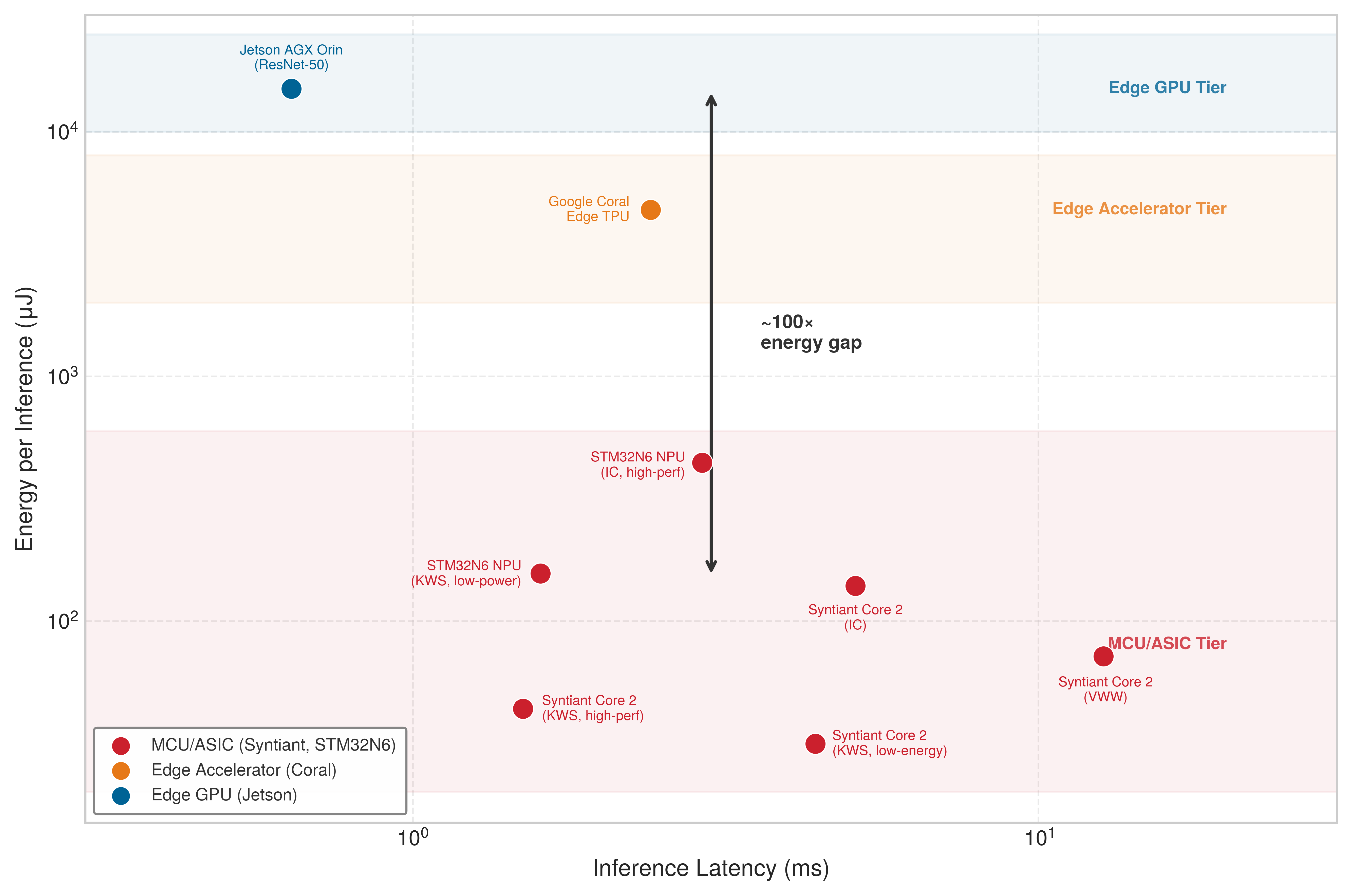
来自 MLPerf Tiny 和厂商官方数据的已发布基准结果使这些硬件层级具体化。图 6 绘制了代表性设备的推理延迟与每次推理能耗曲线，揭示了三个彼此分离约 100$\times$ 倍能耗的硬件层级簇。专用神经处理器（如 Syntiant Core 2 和 STM32N6 NPU）可在 30 到 160 微焦耳的能耗下实现低于 5 ms 的关键词 spotting，而边缘 GPU（如 Jetson AGX Orin）则以 15 毫焦耳的能耗实现亚毫秒延迟。层级之间约 100$\times$ 倍的能耗差距决定了哪些设备能够在电池供电下运行数月而非数小时，从根本上塑造了设备端学习的可行设计空间。

图 6: **边缘推理格局**：来自 MLPerf Tiny 和官方基准的已发布推理延迟与能耗测量揭示了三个硬件层级，彼此能耗相差约 100$\times$。专用神经处理器（Syntiant、STM32N6）可在 30–160 微焦耳的能耗下实现低于 5 ms 的关键词 spotting，而边缘 GPU（Jetson Orin）则以 15 mJ 的能耗实现亚毫秒延迟。

这些计算限制在实时或电池供电系统中尤为突出：节 1.0.2 中确立的延迟预算会转化为硬性架构约束，它们决定了设备端自适应是否可行，或者基于云端的替代方案是否从架构层面成为必需。更严格的约束在于，自适应不能独占设备。在以智能手机为基础的语音识别器中，设备端自适应必须与主推理任务无缝共存，且不得干扰响应延迟或系统响应性。同样，在可穿戴医疗监测设备中，训练必须在经过精心管理的窗口内以机会式方式发生（通常在活动量较低或充电期间），以保存电池寿命并避免热管理问题。

除原始计算能力之外，这些硬件约束的架构影响还延伸至根本性的系统设计选择。训练操作的内存访问模式与推理任务存在根本性差异：反向传播由于梯度计算和激活缓存，需要 3–5$\times$ 倍的更高内存带宽，由此产生纯计算指标无法捕捉的瓶颈。边缘加速器设计通过专门的硬件特性应对这些挑战。自适应精度数据通路允许在正向传递的 INT4 与梯度计算的 FP16 之间动态切换，从而在功耗预算内同时优化精度与效率。稀疏计算单元通过跳过零梯度来加速选择性参数更新，这一能力对于高效的仅偏置更新和结构化低秩更新至关重要（节 1.2.2.2）。近内存计算架构²⁰通过在权重存储旁执行梯度更新来降低数据搬运成本，从而缓解内存带宽瓶颈。然而，许多边缘加速器从根本上仍是针对推理任务优化的，这为设计用于处理本地自适应独特需求的设备端训练加速器提供了软硬件协同设计的机会。

²⁰ 近内存计算：将处理单元放置在内存阵列旁或内存阵列内部，减少常规架构中往往主导算术能耗的数据搬运[^fn-nearmemory-edge-training]Horowitz (2014年)。TensorDIMM 等近内存加速器设计展示了将张量运算移近内存如何改善内存受限深度学习任务的吞吐量和能耗行为[^fn-nearmemory-edge-training]Kwon 和 Rhu (2018年)。对于边缘训练而言，梯度计算会产生以写为主的访问模式，从而压垮缓存层次结构，这一架构转变可能使某些形式的设备端反向传播更具可行性。

Horowitz, Mark. 2014年. 《1.1 Computing’s energy problem (and what we can do about it)》. 2014 IEEE International Solid-State Circuits Conference Digest of Technical Papers (ISSCC), 10～14. https://doi.org/10.1109/isscc.2014.6757323.

Kwon, Youngeun, 和 Minsoo Rhu. 2018年. 《TensorDIMM: A Practical Near-Memory Processing Architecture for Embeddings and Tensor Operations in Deep Learning》. Proceedings of the 52nd Annual IEEE/ACM International Symposium on Microarchitecture, 740～53. https://doi.org/10.1145/3352460.3358284.

移动内存墙

当移动 NPU 提供令人印象深刻的 TOPS 时，内存墙 所考察的“内存墙”对边缘设备上的大规模模型而言却成为不可逾越的障碍。限制训练更新的同一道带宽墙，在移动语言模型的解码中最为直观：如果权重和 KV 状态无法以足够快的速度流式传输通过内存，那么无论标称的 TOPS 数值多么高，都无法挽救该工作负载。近期分析强调了自回归解码如何将大语言模型（LLM）的推理压力推向内存与互连，而非峰值算术吞吐 (Ma 和 Patterson 2026年)。这种数量级差异十分悬殊：H100 上的数据中心 HBM3 提供 3,350 GB/s 的峰值单向 DRAM 内存带宽，而旗舰移动系统（如 A17 Pro 或 Snapdragon 8 Gen 3 设备）的 LPDDR5X 带宽则接近 64–100 GB/s。

Ma, Xiaoyu, 和 David Patterson. 2026年. Challenges and Research Directions for Large Language Model Inference Hardware. No. 5. 卷 59. https://doi.org/10.1109/mc.2026.3652916.

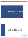
数据中心高带宽内存（HBM）的带宽比移动内存带宽快约 34 倍。

30–50$\times$ 倍的带宽差距意味着，即使模型能够装入移动 RAM，其生成 token 的速度也会比数据中心 GPU 慢 30–50$\times$ 倍。因此，设备端 LLM 服务需要采用激进的量化（INT4，甚至 INT2）作为带宽生存策略，而不仅仅是一种容量优化。将模型规模缩减 8$\times$ 倍，实际上等效地提高了相对带宽，从而使移动硬件上的交互式生成速度成为可能。

Systems Perspective 1.2: 为什么带宽而非 TOPS 才是约束性瓶颈

带宽差距之所以构成约束，是因为每个生成的 token 都需要将模型的权重从内存流式传输到计算单元，因此铁律中的数据项 $(D_{\text{vol}} / \text{BW})$ 在权重超出片上缓存时始终主导计算项；对于移动级硅片上的十亿参数模型，权重确实超出片上缓存。这也解释了为何量化缩减的是 $D_{\text{vol}}$，而非每个 token 的算术量。

由此得出的实用推论是：在为 Transformer 解码排序边缘加速器选项时，衡量标准应是芯片能够持续供给其封装内内存的 GB/s，而非其规格表上的峰值 TOPS。在移动级硅片上，这两者可以相差数个数量级。

边缘硬件集成挑战

除了模型、数据和计算各自的独立约束之外，设备端学习系统还必须应对移动计算底层物理：功耗耗散、热限制和能量预算。这些物理约束是根本性的设计驱动因素，决定了设备端学习算法的整个可行空间。

能量与热约束分析

能量管理与热管理是设备端学习系统设计中最具挑战性的方面，因为它们直接影响用户体验与设备使用寿命。移动设备运行在严格的功耗预算之下，该预算从根本上决定了可行的模型复杂度与训练调度。

Napkin Math 1.1: 电池耗电：边缘学习的代价

问题：一个团队正在为智能手机上的个性化语音助手设计后台微调任务。该训练任务消耗 4.5 W，完成需要 30 minutes。如果手机剩余 15 Wh 电量，这次“隐形”更新会消耗用户多少电量？

数学：

总能耗：4.5 W $\times$ 0.5 h = 2.25 Wh。
电池影响：2.25 Wh/15 Wh = 15 percent。

系统洞察：为后台任务消耗用户 15 percent 的电量，严重违反移动端用户体验原则——相当于损失一小时屏幕常亮时间。这就是为什么设备端训练通常受到机会式调度 的约束：只有当设备处于充电状态、连接 Wi-Fi 且热稳定性良好时，才运行该任务。面向边缘的设计，必须像对待模型的精度预算一样严格地尊重用户的能量预算。

这个电池计算是更广泛能量约束在本地边缘学习中的版本：训练必须适配用户的能量预算，而不只是模型的精度目标。因此，生产设计必须在调度时考虑能耗，比较本地计算与通信开销，并在用户设备无法吸收该更新时推迟学习。

该决策可以表示为后台工作准入条件。设 $E_{\text{update}}$ 为一次自适应窗口预测的能耗，$E_{\text{slack}}$ 为策略允许、直到下一次充电机会之前的能耗，$P_{\text{device}}$ 为当前持续功率，$P_{\text{update}}$ 为自适应增量，$P_{\text{thermal}}$ 为热可持续上限。设 $L_{\text{fg}}$ 为实测前台延迟，$\Delta L_{\text{fg}}^{\text{wc}}$ 为并发自适应下的最差情况延迟增加量，$L_{\text{deadline}}$ 为前台截止时间。运行时仅当

\[ E_{\text{update}} \le E_{\text{slack}} \quad \land \quad P_{\text{device}} + P_{\text{update}} \le P_{\text{thermal}} \quad \land \quad L_{\text{fg}} + \Delta L_{\text{fg}}^{\text{wc}} \le L_{\text{deadline}}. \tag{1}\]

Charging can enlarge the energy allowance, but it does not waive the thermal or foreground-latency tests. The quantities must come from device- and workload-specific profiling, and the runtime must revoke admission when the measured envelope changes. Shorter update windows, a lower duty cycle, or a smaller trainable parameter set can make a rejected update feasible; allowing background learning to consume the foreground deadline cannot.

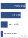
Device memory spans about 15,000 times, phone to microcontroller.

Memory hierarchy optimization

Complementing the thermal and power challenges, memory hierarchy constraints create another fundamental bottleneck that shapes on-device learning system design. The constraint-amplification analysis shows that these limitations affect both static model storage and the dynamic memory requirements during training, often pushing systems beyond their practical limits.

The device memory hierarchy spans several orders of magnitude across different device classes, each presenting distinct constraints for on-device learning. A flagship phone provides about 8 GB total system memory, but only part of that remains available for application workloads after accounting for operating system requirements and background processes. Budget Android devices operate with about 4 GB total system memory, leaving roughly 1 GB–2 GB available for ML workloads after OS overhead consumes significant resources. IoT embedded systems provide 64 MB–1 GB total memory that must be shared between system tasks and application data, creating severe constraints for any learning algorithms. Microcontrollers offer only 256 KB–2 MB SRAM, requiring extreme optimization and careful memory management that fundamentally limits the complexity of models that can adapt on such platforms.

The memory expansion during training creates particularly acute challenges that often determine system feasibility. Standard backpropagation requires caching intermediate activations for each layer during the forward pass, which are then reused during gradient computation in the backward pass, creating substantial memory overhead. A MobileNetV2-scale model that fits comfortably for inference can exceed the available memory budget once activations, gradients, and optimizer state are included, making training impossible without aggressive optimization. Quantization, pruning, and distillation can each reduce model footprint or update cost (Jacob 等 2018年; Han 等 2015年; Hinton 等 2015年), but their gains are workload-specific and do not combine automatically. These techniques must be validated together to achieve the compression required for practical deployment.

Han, Song, Jeff Pool, John Tran, 和 William J. Dally. 2015年. 《Learning both Weights and Connections for Efficient Neural Networks》. Advances in Neural Information Processing Systems 28 (NeurIPS 2015), 1135～43.

Hinton, Geoffrey, Oriol Vinyals, 和 Jeff Dean. 2015年. 《Distilling the Knowledge in a Neural Network》. arXiv preprint.

Cache optimization therefore becomes critical for achieving acceptable performance with constrained memory pools. Modern mobile SoCs feature complex memory hierarchies with L1 cache (32–64 KB), L2 cache (1–8 MB), and system memory (4–16 GB) that exhibit 10–100$\times$ latency differences between levels, creating severe performance cliffs when working sets exceed cache capacity. Training workloads that exceed cache capacity face dramatic performance degradation due to memory bandwidth bottlenecks that can slow training by orders of magnitude. Successful on-device learning systems must carefully design data access patterns to maximize cache hit rates, often requiring specialized memory layouts that group related parameters for spatial locality, carefully sized mini-batches that fit entirely within cache constraints, and sophisticated gradient accumulation strategies that minimize expensive memory bus traffic.

The memory bandwidth limitations become particularly acute during training. While inference workloads primarily read model weights sequentially, training requires bidirectional data flow for gradient computation and weight updates. This increased memory traffic can saturate the memory subsystem, creating bottlenecks that limit training throughput regardless of computational capacity. Advanced implementations employ techniques such as gradient checkpointing²¹ to trade computation for memory (Chen 等 2016年), and mixed-precision training to reduce bandwidth requirements while maintaining numerical stability.

²¹ Gradient Checkpointing: Trades computation for memory by recomputing selected intermediate activations during the backward pass instead of storing all of them. The general checkpointing result is sublinear activation memory at the cost of extra forward computation (Chen 等 2016年). On edge devices where memory is the binding constraint, this trade-off can make the difference between a model that fits in 2 GB RAM and one that requires 8 GB, but the exact memory and compute factors are architecture- and schedule-dependent.

Mobile AI accelerator optimization

Accelerator choice matters less as a peak-TOPS comparison than as a question of which training primitive the hardware can sustain. Fixed-precision inference engines favor inference-heavy adaptation, programmable vector units make compact backpropagation more plausible, and tight framework integration lowers federated coordination overhead. The architectural differences between these accelerators shape the design space for on-device training algorithms.

Flagship-class mobile accelerators should be read as different adaptation envelopes, not as a peak-TOPS ranking. Flagship-class mobile NPUs provide tens of TOPS of peak performance, with 35 TOPS serving here as a generic high-end reference point rather than a single named chip. Apple’s Neural Engine is optimized primarily for CoreML inference patterns with limited training support, making it well suited for inference-heavy adaptation techniques. Qualcomm’s Hexagon digital signal processor (DSP) in the Snapdragon 8 Gen 3 achieves 45 TOPS with flexible precision support and programmable vector units, enabling mixed-precision training workflows that can adapt precision dynamically based on training phase and memory constraints. Google’s Tensor processing unit (TPU) in the Pixel 8 is optimized specifically for TensorFlow Lite operations with strong INT8 performance and tight integration with federated learning frameworks, reflecting a software-stack focus on distributed learning scenarios. The energy-efficiency gap explains why dedicated neural processing units are essential: NPUs achieve 1–5 TOPS per watt vs. general-purpose CPUs at just 0.1-0.2 TOPS per watt, representing a 5–50$\times$ efficiency advantage that makes the difference between feasible and infeasible on-device training.

Each accelerator implies different learning paradigms. Apple’s Neural Engine excels at fixed-precision inference but provides limited support for dynamic precision gradient computation, making it better suited for inference-heavy adaptation techniques like few-shot learning. Programmable DSPs offer greater training flexibility through vector units and mixed-precision arithmetic, enabling backpropagation on compact models when the software stack exposes the needed operators. Mobile TPU-class accelerators integrate tightly with framework runtimes and federated learning tooling, reducing the systems overhead of local training and update coordination.

These per-vendor envelopes inherit the same training-specific access patterns and hardware features discussed under 节 1.1.4: the write-heavy gradient flow, the adaptive-precision datapaths, sparse-update units, and near-memory compute that distinguish a training-capable accelerator from an inference-only one. The consequence for design is that architecture selection here is not a peak-throughput choice; it influences everything from model quantization strategies and gradient computation approaches to federated communication protocols and thermal management policies.

Holistic resource management strategies

The constraint analysis in this section reveals three challenge categories that define the on-device learning design space, and each category drives a corresponding solution pillar. Resource amplification, where training increases memory requirements by 4–12$\times$, computational costs by 2–3$\times$, and energy consumption proportionally, necessitates Model Adaptation approaches that reduce the scope of parameter updates while preserving learning capability. Information scarcity, including limited local datasets, non-IID distributions, privacy restrictions on data sharing, and minimal supervision, drives data efficiency solutions that extract maximum learning signal from minimal examples. Coordination challenges, such as device heterogeneity, intermittent connectivity, distributed validation complexity, and scalability requirements, motivate federated coordination mechanisms that enable privacy-preserving collaboration across device populations.

表 1 reveals how this on-device learning constraint-solution mapping creates a systematic engineering framework: Model Adaptation addresses memory and compute limits through selective parameter updates, Data Efficiency maximizes learning from scarce private samples, and Federated Coordination enables privacy-preserving collaboration. Rather than viewing these as independent techniques, robust systems orchestrate all three approaches to create coherent adaptive systems that operate effectively within edge constraints.

表 1: Constraint-Solution Mapping: The three fundamental constraint categories in on-device learning each drive corresponding solution approaches through direct necessity.

Constraint Category	Key Challenges	Solution Approach
Resource Amplification	• Training workloads (4–12$\times$ memory) • Memory limitations • Power constraints	Model Adaptation • Parameter-efficient updates • Selective layer fine-tuning • Low-rank adaptations
Information Scarcity	• Limited local datasets • Non-IID distributions	Data Efficiency
	• Privacy restrictions	• Few-shot learning
		• Meta-learning • Transfer learning
Coordination Challenges	• Device heterogeneity • Intermittent connectivity • Distributed validation complexity • Scalability requirements	Federated Coordination • Federated averaging and asynchronous aggregation • Secure aggregation and differential privacy • Client selection and straggler handling

Each solution pillar extends compression and distributed-systems tools to address a specific constraint category. No single pillar suffices on its own, but their integration creates systems capable of meaningful adaptation within the severe constraints of edge deployment environments.

Model Adaptation

Personalizing a billion-parameter model on a smartwatch with 500 MB of total system memory is impossible without abandoning the goal of updating the complete model. Instead of updating the whole model, the system freezes the vast majority of the network and trains only a compact, strategically placed set of parameters. This is the essence of resource-efficient model adaptation.

Napkin Math 1.2: The hidden cost of personalization

Problem: A team is deploying a 10M parameter vision model to a smartphone with support for 10 different “User Contexts” (Home, Office, Car, etc.). If a full fine-tuned model requires 40 MB, how much storage does using residual adapters save instead?

Math:

Full Fine-Tuning: 10 contexts $\times$ 40 MB = 400 MB.
Adapter Approach: (1 $\times$ 40 MB backbone) + (10 $\times$ 200 KB adapters) $\approx$ 42 MB.
Storage Savings: 400 MB/42 MB $\approx$ 9.5× total device storage reduction.
Per-Context Efficiency: 40 MB/0.2 MB = 200×.

Systems insight: Personalization is a storage density problem. On a device with limited flash memory, storing 10 versions of the same 40 MB model quickly consumes 400 MB. Sharding the model into a frozen backbone and dynamic adapters reduces the marginal cost of a new user context by 200×. In the edge fleet, modularity is the only way to scale intelligence without exhausting the physical hardware.

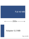
Adapters make per-user personalization cheap vs. full model copies.

The engineering challenge centers on navigating a fundamental trade-off space: adaptation expressivity vs. resource consumption. At one extreme, updating all parameters provides maximum flexibility but exceeds edge device capabilities. At the other extreme, no adaptation preserves resources but fails to capture user-specific patterns. Effective on-device learning systems must operate in the middle ground, selecting adaptation strategies based on three key engineering criteria:

Resource envelope determines which adaptation approaches are feasible. A tiny wearable-class device with 1 MB RAM requires fundamentally different strategies than a smartphone with 8 GB.
User-specific variation determines how much adaptation complexity the system needs. Simple preference learning may require only bias updates, while complex domain shifts demand more sophisticated approaches.
Systems integration determines whether the adaptation technique can fit existing inference pipelines, federated coordination protocols, and operational monitoring systems for model deployment and lifecycle management.

The selection of adaptation techniques follows the same logic, starting with lightweight approaches (节 1.2.1) and progressing to more expressive but resource-intensive methods (节 1.2.3). Each technique represents a different point in the engineering trade-off space.

On top of the compression baseline established in 节 1.1, model adaptation adds a second move: complete model retraining is neither necessary nor feasible at the edge, so systems use pretrained representations strategically and adapt only the minimal parameter subset required to capture local variations: preserve what works globally, adapt what matters locally. Those three criteria turn adaptation into a device-matching decision. Weight freezing fits severe memory limits by updating only bias terms or final layers. Structured updates use low-rank and residual adaptations when the device can afford more expressiveness but not full fine-tuning. Sparse updates reserve scarce training capacity for the parameters with the highest adaptation value.

Weight freezing

The most direct approach to on-device learning is to freeze the majority of a model’s parameters and adapt only a minimal subset. Bias-Only Adaptation holds all weights fixed and updates only the bias terms (scalar offsets applied after linear or convolutional layers). The constraint reduces trainable parameters by 100–1000$\times$, simplifies memory management during backpropagation, and helps mitigate overfitting when training data is sparse or noisy.

Consider a standard neural network layer: \[ y = W x + b \] where $\mathbf{W} \in \mathbb{R}^{m \times n}$ is the weight matrix, $b \in \mathbb{R}^m$ is the bias vector, and $x \in \mathbb{R}^n$ is the input. In full training, gradients are computed and applied to both $W$ and $b$. In bias-only adaptation, the system freezes the weight tensor ($\Delta W = 0$) and computes gradients exclusively for the bias: \[ W \leftarrow W, \quad b \leftarrow b - \eta \frac{\partial \mathcal{L}}{\partial b} \]

This reduces the number of stored gradients and optimizer states, enabling training to proceed under memory-constrained conditions. On embedded devices that lack floating-point units, this reduction enables on-device learning. 代码 1 makes the constraint explicit: all convolutional and fully connected weights remain frozen, while only bias terms adapt to local data.

列表 1: Bias-Only Adaptation: Freezes model parameters except for biases to reduce memory usage and allow on-device learning.

# Freeze all parameters
for name, param in model.named_parameters():
    param.requires_grad = False

# Enable gradients for bias parameters only
for name, param in model.named_parameters():
    if "bias" in name:
        param.requires_grad = True

This pattern ensures that only bias terms participate in the backward pass and optimizer update, simplifying the training process while maintaining adaptation capability. This is valuable when adapting pretrained models to user-specific or device-local data where the core representations remain relevant but require calibration.

The practical effectiveness of this approach is demonstrated by Tiny Transfer Learning (TinyTL) (Cai 等 2020年), a framework explicitly designed to enable efficient adaptation of deep neural networks on microcontrollers and other severely memory-limited platforms. Rather than updating all network parameters during training (impossible on such constrained devices), TinyTL strategically freezes both the convolutional weights and the batch normalization statistics, training only the bias terms and, in some cases, lightweight residual components. This architectural constraint creates a profound shift in memory requirements during backpropagation, since the largest memory consumers (intermediate activations) no longer need to be stored for gradient computation across frozen layers.

图 7 visualizes this architectural impact by contrasting standard training with the TinyTL approach. Where conventional backpropagation requires storing activations across all layers, TinyTL freezes backbone weights and batch normalization statistics, training only the final classifier and lightweight bias modules. This eliminates the need to store activations for frozen layers, making adaptation possible within the severe memory constraints established earlier.

图 7: TinyTL memory optimization: The panels compare conventional fine-tuning with TinyTL. Conventional backpropagation stores activations across all layers, whereas TinyTL freezes backbone weights and trains only bias terms and lightweight residual modules, reducing memory requirements for on-device adaptation.

The memory reduction is useful only when the frozen backbone remains expressive enough for the downstream task. The bias terms allow for minor but meaningful shifts in model behavior, particularly for personalization tasks. When domain shift is more significant, TinyTL can optionally incorporate small residual adapters to improve expressivity, all while preserving the system’s tight memory and energy profile.

These design choices allow TinyTL to reduce training memory usage by 10$\times$. For instance, adapting a MobileNetV2 model using TinyTL can reduce the number of updated parameters from over 3 million to fewer than 50,000.²² Combined with quantization, this allows local adaptation on devices with only a few hundred kilobytes of memory, making on-device learning truly feasible in constrained environments.

²² TinyTL Memory Savings: The approximately 68× trainable-parameter reduction (3.4 M to 50 K) collapses MobileNetV2 training memory from approximately 20 MB (weights + activations in FP32) to approximately 600 KB, fitting within a 1 MB microcontroller budget. Real deployments on STM32H7 achieve 85 percent of full fine-tuning accuracy while completing updates in approximately 30 seconds vs. 8 minutes, demonstrating that bias-only adaptation trades expressivity for feasibility on the most constrained hardware.

图 8 breaks down this memory profile, contrasting the ~2,100 KB footprint of standard fine-tuning against the ~390 KB footprint of TinyTL relative to the 512 KB on-chip SRAM budget of typical microcontrollers.

图 8: TinyTL memory breakdown: Comparison of training memory breakdown between standard fine-tuning and TinyTL on microcontroller hardware. Standard backpropagation requires storing intermediate activations that exceed the 512 KB SRAM ceiling, whereas TinyTL operates comfortably within SRAM by eliminating backbone activation caching.

Structured parameter updates

While weight freezing provides computational efficiency and clear memory bounds, it severely limits model expressivity by constraining adaptation to a small parameter subset. When bias-only updates prove insufficient for capturing complex domain shifts or user-specific patterns, residual and low-rank techniques provide a middle ground between the extreme efficiency of weight freezing and the full expressivity of unrestricted fine-tuning. Rather than modifying existing parameters, these methods extend frozen models by adding small trainable components, such as residual adaptation modules (Houlsby 等 2019年) or low-rank parameterizations (Hu 等 2021年). The main body of the network remains fixed, while only the added components are optimized, so the model can respond to new data without giving up the memory and compute bounds that make on-device adaptation feasible.

Houlsby, Neil, Andrei Giurgiu, Stanislaw Jastrzebski, Bruna Morrone, Chloé de Laroussilhe, Andrea Gesmundo, Mohammad Attariyan, 和 Sylvain Gelly. 2019年. 《Parameter-efficient transfer learning for NLP》. International Conference on Machine Learning (ICML), 2790～99.

Adapter-based adaptation

A common implementation involves inserting residual adapters, which are small residual bottleneck layers, between existing layers in a pretrained model. Consider a hidden representation $h$ passed between layers. A residual adapter introduces a transformation: \[ h′ = h + A(h) \] where $A(\cdot)$ is a trainable function, typically composed of two linear layers with a nonlinearity: \[ A(h) = W_2 \, \sigma(W_1 h) \] with $W_1 \in \mathbb{R}^{r \times d}$ and $W_2 \in \mathbb{R}^{d \times r}$, where $r \ll d$. This bottleneck design ensures that only a small number of parameters are introduced per layer.

The adapters act as learnable perturbations on top of a frozen backbone. Because they are small and sparsely applied, they add negligible memory overhead, yet they allow the model to shift its predictions in response to new inputs.

Low-rank techniques

Another efficient strategy is to constrain weight updates themselves to a low-rank structure. Rather than updating a full matrix $\mathbf{W}$, the update is approximated as: \[ \Delta \mathbf{W} \approx \mathbf{U} \mathbf{V}^\top \] where $\mathbf{U} \in \mathbb{R}^{m \times r}$ and $\mathbf{V} \in \mathbb{R}^{n \times r}$, with $r \ll \min(m,n)$. This reduces the number of trainable parameters from $mn$ to $r(m + n)$.

The mathematical intuition behind this decomposition connects to fundamental linear algebra principles: any matrix can be expressed as a sum of rank-one matrices through singular value decomposition. Constraining updates to low rank (typically $r = 4$ to $16$) captures a restricted set of variation modes while reducing parameters. For a typical transformer layer with dimensions $768{\times}768$, full fine-tuning requires updating 589,824 parameters. With rank-4 decomposition, only $768{\times}4{\times}2 =$ 6,144 parameters are updated, a 99 percent reduction. Whether this retains most of the adaptation quality depends on the task, rank, and base model; low-rank adaptation (LoRA) reports that low-rank adapters can match or approach full fine-tuning on several transformer adaptation benchmarks (Hu 等 2021年).

During adaptation, the new weight is computed as: \[ W_{\text{adapted}} = W_{\text{frozen}} + U V^\top \]

This formulation is commonly used in LoRA,²³ originally developed for transformer models (Hu 等 2021年) but broadly applicable across architectures. From a systems engineering perspective, LoRA makes the trainable adapter the artifact that can be stored, transmitted, scheduled, and rolled back separately from the frozen base model.

²³ LoRA (Low-Rank Adaptation): Hu 等 (2021年) learn rank-$r$ decomposition matrices $\mathbf{A}$ and $\mathbf{B}$ instead of updating full weight matrices, reducing trainable parameters by 100–10,000$\times$ while maintaining much of the adaptation quality. For on-device learning, this compression is decisive, but it affects adapter state rather than the full model footprint: a model with 7B parameters has about a 14 GB FP16 weight footprint before gradients, optimizer state, and activations, while rank 16 LoRA can reduce the trainable adapter parameters to tens or hundreds of megabytes. Practical phone deployment still requires storing, quantizing, or offloading the frozen base model.

Hu, Edward J., Yelong Shen, Phillip Wallis, Zeyuan Allen-Zhu, Yuanzhi Li, Shean Wang, Lu Wang, 和 Weizhu Chen. 2021年. 《LoRA: Low-Rank Adaptation of Large Language Models》. arXiv preprint arXiv:2106.09685.

图 9 illustrates the dual-path architecture of Low-Rank Adaptation (LoRA), separating the frozen pretrained matrix $W_0$ from the low-rank down- and up-projection matrices $A$ and $B$.

图 9: LoRA architecture and parameter efficiency: The input $x$ passes through both the frozen base weight matrix $W_0$ and the low-rank trainable adapter path consisting of down-projection $A$ and up-projection $B$. At inference, the adapter weights can be folded directly into the base weights with zero additional latency.

Consider a mobile deployment where a language model with 7B parameters has a 14 GB FP16 weight footprint, before accounting for the additional gradients, optimizer states, and activations required by full fine-tuning. That footprint is impossible on smartphones with about 8 GB total memory unless the base model is aggressively quantized, partitioned, or offloaded. LoRA with rank 16 can reduce the trainable adapter parameters to tens or hundreds of megabytes, making local adaptation plausible only when the frozen base model is handled separately.

LoRA’s efficiency becomes critical in intermittent connectivity scenarios. A full model update over cellular networks would require a 14 GB download and corresponding data-plan cost, while the tier-profile adapter update is 50 MB. Small adapter updates can synchronize in under a minute on good mobile links; larger adapter updates typically require LTE or Wi-Fi for sub-minute coordination and may take minutes on 3G. This is still dramatically more practical than hours-long full model transfers.

A device-tiered deployment can use different adapter configurations based on device capabilities. Flagship phones use wider bottlenecks for higher expressivity, mid-range devices use moderate bottlenecks for balanced performance, and budget devices use narrow bottlenecks to stay within about 2 GB memory limits. These residual adapter modules can be implemented efficiently on edge devices, particularly when the down-projection and up-projection matrices are small and fixed-point representations are supported. 代码 2 implements this low-rank adapter pattern as a residual bottleneck, showing how a compact down/up projection adds trainable capacity without updating the frozen backbone.

Example 1.1: On-device keyboard learning

Scenario: Large-scale mobile keyboard systems (e.g., Gboard) adapt next-word prediction models locally across hundreds of millions of mobile devices (McMahan 等 2017年).

Diagnosis: Local training risks OS process eviction and user disruption if memory $M_{\text{peak}} \ge 50\text{ MB}$ or battery drops. The pipeline gates training to run strictly when the device is idle, charging, and on Wi-Fi, using quantized update vectors to minimize network payload $D_{\text{vol}} / \text{BW}$.

Systems lesson: On-device learning is viable only when local resource bounds ($M_{\text{peak}}$, $E_{\text{battery}}$), network bandwidth ($D_{\text{vol}} / \text{BW}$), and differential privacy are engineered together as an end-to-end systems protocol.

Returning to the adapter mechanism, 代码 2 shows the residual bottleneck that makes the memory savings concrete: the frozen backbone remains untouched, while only the down-projection and up-projection weights are trained.

列表 2: Residual Bottleneck Adapter: The code implements a compact adapter module with down-projection and up-projection layers, reducing trainable parameter count while enabling efficient model adaptation on edge devices.

import torch.nn as nn


class Adapter(nn.Module):
    def __init__(self, dim, bottleneck_dim):
        super().__init__()
        # Project from full dimension to bottleneck (e.g., 768 -> 16)
        self.down = nn.Linear(
            dim, bottleneck_dim
        )  # W1: learns compression
        # Project back to original dimension (e.g., 16 -> 768)
        self.up = nn.Linear(
            bottleneck_dim, dim
        )  # W2: learns expansion
        self.activation = nn.ReLU()

    def forward(self, x):
        # Residual connection: original + low-rank adaptation
        # Only adapter params trained; base model frozen
        return x + self.up(self.activation(self.down(x)))

This adapter adds a small residual transformation to a frozen layer. When inserted into a larger model, only the adapter parameters are trained.

Edge personalization

Adapters enable an efficient multi-tenant architecture for edge intelligence, where a single frozen backbone supports multiple personalized contexts. Consider a 10M parameter vision model deployed on a smartphone with 8 GB RAM. Full fine-tuning would require storing a separate 40 MB copy of the model weights for each personalization context (home, office, outdoor), rapidly consuming the device’s storage. A rank-64 adapter introduces only approximately 50,000 parameters (roughly 200 KB) per context—a 200$\times$ reduction in storage. This efficiency allows the device to store dozens of specialized adapters that share the same frozen backbone, swapping them dynamically based on the user’s location or activity.

This Adapter Switching pattern transforms the smartphone from a static inference engine into a context-aware learning system. When the user enters a low-light environment, the system can load the appropriate adapter into the vision pipeline instead of replacing the entire backbone. The modularity extends naturally to federated learning: in the 10M-parameter example introduced earlier in this section, transmitting a 200 KB adapter is far cheaper than transmitting a 40 MB full-model update over a bandwidth-constrained cellular connection. Residual-adapter studies show that small trainable modules can adapt a shared visual backbone across multiple visual domains (Rebuffi 等 2017年), making them a useful design point between personalization quality and system resources. The frozen backbone helps preserve general visual representations, while adapters provide a bounded place for user- or context-specific updates without exposing the entire model to catastrophic forgetting, the loss of previously learned general behavior when new updates overwrite it (formalized in 节 1.3.2 later in this chapter).

Rebuffi, Sylvestre-Alvise, Hakan Bilen, 和 Andrea Vedaldi. 2017年. 《Learning multiple visual domains with residual adapters》. Advances in Neural Information Processing Systems (NeurIPS) 30.

In smartphone camera pipelines, environmental lighting, user preferences, and lens distortion vary between users. A shared model can be frozen and fine-tuned per-device using a few residual modules, allowing lightweight personalization without destabilizing the base model. In voice-based systems, adapter modules reduce word error rates in personalized speech recognition without retraining the full acoustic model. They also allow easy rollback or switching between user-specific versions—a critical operational capability when local adaptation occasionally degrades rather than improves performance.

Performance vs. resource trade-offs

Selecting the right adaptation strategy requires quantitative analysis of the resource-expressivity spectrum. For a 10M parameter model, the trade-offs are concrete. Bias-only updates are the most efficient, requiring just 50 KB of trainable parameters and negligible compute overhead, but they struggle to adapt to structural domain shifts like changing sensor geometries or new object categories. At the other extreme, full fine-tuning offers maximum expressivity but demands 40 MB or more of gradients and optimizer states, making it infeasible for background training on typical mobile devices. LoRA and residual adapters occupy the strategic middle ground: the rank-64 LoRA configuration described in 节 1.2.2.3 requires roughly 200 KB of trainable memory, while a standard residual adapter needs a few megabytes.

The decision between LoRA and residual adapters often hinges on inference latency constraints. LoRA matrices can be mathematically merged into the frozen backbone weights during inference $(\mathbf{W}_{\text{final}} = \mathbf{W}_{\text{frozen}} + \mathbf{U} \mathbf{V}^\top)$, resulting in zero additional inference latency. This makes LoRA ideal for latency-critical paths like real-time video processing where every millisecond matters. Residual adapters, conversely, remain distinct modules ($y = f(x) + \text{Adapter}(x)$), adding 1–3 percent to inference latency due to the extra forward pass through the adapter layers. However, this separation enables the hot-swapping capability described earlier: switching adapters requires loading only the small adapter weights rather than recomputing merged matrices.

Implementing these adaptation techniques requires system-level support for dynamic computation graphs and the ability to selectively inject trainable parameters. Not all deployment environments or inference engines support such capabilities natively. TensorFlow Lite and Open Neural Network Exchange (ONNX) Runtime Mobile provide support for adapter-style architectures, but custom inference stacks on microcontrollers may require manual implementation of the adapter forward pass.

System architects should apply a device-tier framework to this decision. On flagship phones (Tier 1) with dedicated Neural Engines and 8 GB of RAM or more, residual adapters provide a strong balance of modularity and speed, enabling context-aware switching with minimal latency impact. On mid-range devices (Tier 2) with 1 GB up to that ceiling, LoRA is attractive because weight merging eliminates runtime overhead entirely. For ultra-constrained IoT endpoints (Tier 3) with less than 1 GB RAM, bias-only updates may be the only practical option. This tiered approach ensures that the adaptation mechanism matches the physical reality of the hardware, preventing thermal throttling while delivering meaningful personalization at each capability level.

Checkpoint 1.2: Edge personalization

Verify understanding of efficient on-device adaptation:

Adapter switching: Explain why Adapter Switching is more storage-efficient than maintaining separate full-model copies for different user contexts.
Adapter size: Compare the size of a rank-64 adapter to a standard 10M parameter vision model.
Residual vs. LoRA: Identify the deployment tier (Tier 1, 2, or 3) where Residual Adapters are preferred over LoRA and justify the choice.
Adapter bandwidth: Evaluate the claim that transmitting adapter weights in federated learning consumes more bandwidth than transmitting the entire model.

Sparse updates

Sparse updates are the highest-expressivity end of the model adaptation hierarchy. Instead of adding new parameters or choosing a fixed subset in advance, the system dynamically identifies which existing parameters provide the greatest adaptation benefit for a specific task or user. This preserves more of full fine-tuning’s flexibility while keeping the update footprint small enough for edge deployment.

The sparse-update decision goes beyond updating fewer parameters. Training remains resource-intensive even after model-adaptation techniques restrict learning to a small subset. Sparse updating addresses the remaining cost by selecting only task-relevant parameters, reducing memory and compute while preserving meaningful personalization.

The key insight is that layers do not contribute equally to local performance gains. If the system can identify the minimal subset with the highest adaptation value, it can spend scarce training capacity where it changes the model’s behavior most.

Sparse update design

Let a neural network be defined by parameters $\theta = \{\theta_1, \theta_2, \ldots, \theta_{N_L}\}$ across $N_L$ layers. In standard fine-tuning, gradients are computed and updates are performed on all parameters: \[ \theta_i \leftarrow \theta_i - \eta \frac{\partial \mathcal{L}}{\partial \theta_i}, \quad \text{for } i = 1, \ldots, N_L \]

In task-adaptive sparse updates, the system selects a small subset $\mathcal{S} \subset \{1, \ldots, N_L\}$ such that only parameters in $\mathcal{S}$ are updated: \[ \theta_i \leftarrow \begin{cases} \theta_i - \eta \frac{\partial \mathcal{L}}{\partial \theta_i}, & \text{if } i \in \mathcal{S} \\ \theta_i, & \text{otherwise} \end{cases} \]

The challenge lies in selecting the optimal subset $\mathcal{S}$ given memory and compute constraints. A principled strategy is contribution analysis, an empirical method that estimates how much each layer contributes to downstream performance improvement. For example, one can measure the marginal gain from updating each layer independently:

Freeze the entire model.
Unfreeze one candidate layer.
Finetune briefly and evaluate improvement in validation accuracy.
Rank layers by performance gain per unit cost (e.g., per KB of trainable memory).

This layer-wise profiling yields a ranking from which $\mathcal{S}$ can be constructed subject to a memory budget.

A concrete example is TinyTrain, a method designed to allow rapid adaptation on-device (Kwon 等 2024年). TinyTrain combines offline preparation with a task-adaptive sparse-update method that dynamically selects layers or channels to update using user data, memory limits, and compute limits. At runtime, the system updates only the selected subset rather than treating the whole network as trainable.

In implementation, selective layer updating turns the ranking into requires_grad decisions or equivalent graph masks. 代码 3 extends this pattern to profiling-driven layer selection, demonstrating how hardware profiling determines which layers to update based on contribution scores and memory constraints.

列表 3: Selective Layer Updating: This technique allows fine-tuning specific layers of a pretrained model while keeping others frozen, optimizing computational resources for targeted improvements. Source: PyTorch Documentation.

# Selective layer update based on contribution analysis
# Layers selected via profiling: conv2 and fc have highest
# accuracy-per-KB impact for this task

for name, param in model.named_parameters():
    if "conv2" in name or "fc" in name:
        param.requires_grad = True  # Train high-impact layers
    else:
        param.requires_grad = False  # Freeze low-impact layers

# Result: ~10% of params trainable, ~60% of adaptation quality
# Memory savings: gradient storage only for selected layers

TinyTrain makes the runtime motivation concrete. Consider a scenario where a user wears an augmented reality headset that performs real-time object recognition. As lighting and environments shift, the system must adapt to maintain accuracy, but training must occur during brief idle periods or while charging. TinyTrain addresses this constraint through task-adaptive sparse updates: the deployment process selects a small update set that fits the device’s memory and compute budget. The approach keeps adaptation fast, energy-efficient, and memory-aware when the target task and device profile match the method’s assumptions.

Task-adaptive sparse updates still introduce system-level trade-offs. Contribution analysis has a nontrivial computational cost even when it occurs during pretraining or initial profiling, so the deployment pipeline must budget for it. Stability also requires attention: if too few parameters are selected for updating, the model may underfit the target distribution, so teams need validation thresholds for the selected subset before deployment. The selection policy must also account for hardware-specific execution costs because some parameters show high contribution scores but prove expensive to update on certain architectures. Despite these trade-offs, task-adaptive sparse updates provide a practical mechanism to scale adaptation across deployment contexts from microcontrollers to mobile devices (Kwon 等 2024年).

Adaptation strategy comparison

Each adaptation strategy offers a distinct balance between expressivity, resource efficiency, and implementation complexity. Bias-only adaptation is the most lightweight approach, updating only scalar offsets in each layer while freezing all other parameters. This reduces memory requirements and computational burden, making it suitable for devices with tight memory and energy budgets. However, its limited expressivity means it is best suited to applications where the pretrained model already captures most of the relevant task features and only minor local calibration is required.

Residual adaptation, often implemented via adapter modules, introduces a small number of trainable parameters into the frozen backbone of a neural network. This allows for greater flexibility than bias-only updates, while still maintaining control over the adaptation cost. Because the backbone remains fixed, training can be performed efficiently and safely under constrained conditions. This method supports modular personalization across tasks and users, making it a favorable choice for mobile settings where moderate adaptation capacity is needed.

Task-adaptive sparse updates offer the greatest potential for task-specific finetuning by selectively updating only a subset of layers or parameters based on their contribution to downstream performance. While this method allows expressive local adaptation, it requires a mechanism for layer selection, through profiling, contribution analysis, or meta-training, which introduces additional complexity. Nonetheless, when deployed carefully, it allows for dynamic trade-offs between accuracy and efficiency, particularly in systems that experience large domain shifts or evolving input conditions. 表 2 contrasts adaptation strategy trade-offs across trainable parameters, memory overhead, expressivity, use-case suitability, and system requirements, revealing how the optimal choice depends on application domain, available hardware, latency constraints, and expected distribution shift.

表 2: Adaptation Strategy Trade-Offs: Table entries characterize three approaches to model adaptation, bias-only updates, residual adapters, and sparse layer updates, by quantifying their impact on trainable parameters, memory overhead, expressivity, suitability for different use cases, and system requirements. These characteristics reveal the inherent trade-offs between model flexibility, computational cost, and performance when deploying machine learning systems in dynamic environments.

Technique	Trainable Parameters	Memory Overhead	Expressivity	Use Case Suitability	System Requirements
Bias-Only Updates	Bias terms only	Minimal	Low	Simple personalization; low variance	Extreme memory/compute limits
Residual Adapters	Adapter modules	Moderate	Moderate to High	User-specific tuning on mobile	Mobile-class SoCs with runtime support
Sparse Layer Updates	Selective parameter subsets	Variable	High (task-adaptive)	Real-time adaptation; domain shift	Requires profiling or meta-training

While freezing weights and training adapters solves the memory bottleneck, it leaves a statistical challenge. Even with a resource-efficient learning mechanism, edge devices rarely possess the thousands of labeled examples required to train adapters from scratch. This constraint introduces the second pillar of on-device learning: data efficiency.

Data Efficiency

A user corrects smartphone keyboard autocorrect perhaps three times a day. The system cannot require 10,000 labeled sentences to train a local language model. Data efficiency at the edge means learning aggressively from a sparse, noisy, and uncurated trickle of implicit user feedback, maximizing the signal extracted from each interaction.

The systems engineering challenge centers on a critical trade-off: data collection cost vs. adaptation quality. Edge devices face severe data acquisition constraints that reshape learning system design in ways not encountered in centralized training. Understanding and navigating these constraints requires systematic analysis of four interconnected engineering dimensions:

Acquisition cost includes user friction, energy consumption, storage overhead, and privacy risk. A voice assistant learning from audio samples must balance improvement potential against battery drain and user comfort with always-on recording.
Collection depth determines whether the system spends limited capacity on broad coverage or detailed examples. A mobile keyboard can collect many shallow typing patterns or fewer detailed interaction sequences, each strategy implying different learning approaches.
Learning urgency determines whether the system must adapt from minimal examples immediately, as in emergency response scenarios, or can accumulate evidence over time, as in user preference learning.
Lifecycle integration determines whether data efficiency techniques fit the model adaptation approaches from 节 1.2, federated coordination (节 1.4), and operational monitoring for model deployment and lifecycle management.

These engineering constraints create a systematic trade-off space where different data efficiency approaches serve different combinations of constraints. Rather than choosing a single technique, successful on-device learning systems typically combine multiple approaches, each addressing specific aspects of the data scarcity challenge.

The strategy choice depends on which scarcity binds first. Few-shot learning fits cases where a few labeled or weakly labeled examples must drive personalization. Streaming updates fit settings where useful data arrives incrementally and cannot be batched in advance. Experience replay spends memory to stabilize continual updates by reusing scarce examples. Data compression reduces the storage cost of those histories so replay and lightweight training remain feasible within edge memory budgets.

Few-shot learning and data streaming

Together, these techniques turn data scarcity into an allocation problem: spend labels, memory, compute, and privacy budget where they produce the most reliable local signal. In conventional machine learning workflows, effective training typically requires large labeled datasets, carefully curated and preprocessed to ensure sufficient diversity and balance. On-device learning, by contrast, must often proceed from only a handful of local examples, collected passively through user interaction or ambient sensing, and rarely labeled in a supervised fashion. These constraints motivate two complementary adaptation strategies: few-shot learning, in which models generalize from a small, static set of examples, and streaming adaptation, where updates occur continuously as data arrives.

Few-shot adaptation is particularly relevant when the device observes a small number of labeled or weakly labeled instances for a new task or user condition (Wang 等 2020年). In such settings, it is often infeasible to perform full finetuning of all model parameters without overfitting. Instead, methods such as bias-only updates, adapter modules, or prototype-based classification are employed to make use of limited data while minimizing capacity for memorization. Let $\mathcal{S} = \{(x_i, y_i)\}_{i=1}^K$ denote a $K$-shot dataset of labeled examples collected on-device. The model update is viable only if three constraints remain bounded:

Wang, Y., Q. Yao, J. T. Kwok, 和 L. M. Ni. 2020年. 《Generalizing From a Few Examples: A Survey on Few-Shot Learning》. ACM Computing Surveys 53 (3): 1～34. https://doi.org/10.1145/3386252.

Gradient work stays small: $K_{\text{steps}} \ll 100$.
Updated parameter count stays compact: $|\theta_{\text{updated}}| \ll |\theta|$.
Prior task knowledge remains preserved, avoiding catastrophic forgetting.

Keyword spotting (KWS) systems are a common target for data-efficient on-device adaptation; Speech Commands provides a standard dataset for training and evaluating limited-vocabulary KWS models under on-device constraints (Warden 2018年). These models are used to detect fixed phrases, including phrases like “Hey Siri”²⁴ or “OK Google”, with low latency and high reliability. A typical KWS model consists of a pretrained acoustic encoder (e.g., a small convolutional or recurrent network that transforms input audio into an embedding space) followed by a lightweight classifier. In commercial systems, the encoder is trained centrally using thousands of hours of labeled speech across multiple languages and speakers. However, supporting custom wake words (e.g., “Hey Jarvis”) or adapting to underrepresented accents and dialects is often infeasible via centralized training due to data scarcity and privacy concerns.

Warden, Pete. 2018年. 《Speech Commands: A Dataset for Limited-Vocabulary Speech Recognition》. arXiv preprint arXiv:1804.03209, 网络首发. https://doi.org/10.48550/arXiv.1804.03209.

²⁴ “Hey Siri” Power Budget: The always-on detector consumes $<1$ mW while monitoring audio continuously, using a compact acoustic model on a low-power always-on processor rather than the main application cores. The constraint envelope is extreme: $<100$ ms detection latency, $<0.1$ false activations per hour, and $>95$ percent true positive rate across accents and noise conditions. Few-shot personalization must improve accuracy within this fixed power and model-size budget, meaning adaptation can tune classifier weights but cannot expand the model.

Few-shot adaptation solves this problem by finetuning only the output classifier or a small subset of parameters, including bias terms, using just a few example utterances collected directly on the device. For example, a user might provide 5–10 recordings of their custom wake word. These samples are then used to update the model locally, while the main encoder remains frozen to preserve generalization and reduce memory overhead. This allows personalization without requiring additional labeled data or transmitting private audio to the cloud.

The approach is computationally efficient and aligned with privacy-preserving design principles. Because only the output layer is updated, often involving a single gradient step or prototype computation, the total memory footprint and runtime compute are compatible with mobile-class devices or even microcontrollers.

Beyond static few-shot learning, many on-device scenarios benefit from streaming adaptation, where models must learn incrementally as new data arrives (Hayes 等 2020年). Streaming adaptation generalizes this idea to continuous, asynchronous settings where data arrives incrementally over time. Let $\{x_t\}_{t=1}^{\infty}$ represent a stream of observations. In streaming settings, the model must update itself after observing each new input, typically without access to prior data, and under bounded memory and compute. The computable loss may come from implicit feedback, pseudo-labels, self-supervised objectives, reconstruction error, or a task-specific proxy rather than explicit human labels. The model update can be written generically as: \[ \theta_{t+1} = \theta_t - \eta_t \nabla \mathcal{L}(x_t; \theta_t) \] where $\eta_t$ is the learning rate at time $t$. This form of adaptation is sensitive to noise and drift in the input distribution, and thus often incorporates mechanisms such as learning rate decay, meta-learned initialization, or update gating to improve stability.

Aside from KWS, practical examples of these strategies abound. In wearable health devices, a model that classifies physical activities may begin with a generic classifier and adapt to user-specific motion patterns using only a few labeled activity segments. In smart assistants, user voice profiles are fine-tuned over time using ongoing speech input, even when explicit supervision is unavailable. Local corrections, repetitions, or downstream task completion can provide implicit signals, but only after the system defines which event counts as feedback and tests its validity. A user may accept a suggestion because it is convenient rather than correct, abandon a task for reasons unrelated to the model, or correct an error that the model itself induced. Production adaptation should therefore separate observed events from inferred labels, retain a nonadapting control cohort, measure delayed outcomes when available, and gate learning when the proxy-to-outcome relationship drifts.

Few-shot and streaming adaptation form the foundation for more advanced memory and replay strategies that address the stability challenges of continuous on-device learning.

Experience replay

Definition 1.2: Catastrophic forgetting

Catastrophic Forgetting is the phenomenon in which a neural network trained sequentially on new tasks or data distributions rapidly loses performance on previously learned tasks, because gradient updates that optimize the new objective overwrite weight configurations that supported the old ones.

Significance: Without explicit mitigation, fine-tuning a deployed classifier on a new domain can sharply reduce prior-task accuracy, even when the new domain is closely related to the old one (Kirkpatrick 等 2017年). This is the central failure mode of on-device and federated learning: every device that adapts locally to its user’s recent data risks erasing the general capabilities the centralized training run paid for, and the loss is invisible until inference encounters out-of-recent-context inputs.
Distinction: Unlike overfitting (a generalization failure on a single fixed task) and distribution shift (a deployment-time mismatch between training and inference data), forgetting is a training-time phenomenon caused by the sequential structure of the update stream itself; the model’s capacity is sufficient, but its weights cannot encode the new objective without disturbing the encoding of the old one.
Common pitfall: A frequent misconception is that a small experience-replay buffer is sufficient protection. Naive replay of 100 to 1,000 stored samples can mask short-horizon forgetting on a held-out validation set yet still degrade rare-class or long-tail performance, because the buffer’s sampling distribution under-represents the tails. Production deployments require capacity-proportional buffers, prioritized replay, or weight-regularization methods such as elastic weight consolidation (节 1.6.2).

Learning the new task erodes accuracy on the old one.

Experience replay addresses catastrophic forgetting in continuous learning scenarios by maintaining a buffer of representative examples from previous learning episodes. This technique, originally developed for reinforcement learning (Mnih 等 2015年), proves essential in on-device learning where sequential data streams can cause models to overfit to recent examples. Here, experience replay addresses the immediate stability need; bio-inspired lifelong learning (节 1.6.2) addresses the same stability problem through local plasticity and consolidation mechanisms.

Unlike server-side replay strategies that rely on large datasets and extensive compute, on-device replay must operate with extremely limited capacity, often with tens or hundreds of samples, and must avoid interfering with user experience (Rolnick 等 2019年). Buffers may store only compressed features or distilled summaries, and updates must occur opportunistically (e.g., during idle cycles or charging). These system-level constraints reshape how replay is implemented and evaluated in the context of embedded ML.

Let $\mathcal{M}$ represent a memory buffer that retains a fixed-size subset of training examples. At time step $t$, the model receives a new data point $(x_t, y_t)$ and appends it to $\mathcal{M}$. A replay-based update then samples a batch $\{(x_i, y_i)\}_{i=1}^{k}$ from $\mathcal{M}$ and applies a gradient step: \[ \theta_{t+1} = \theta_t - \eta \nabla_\theta \left[ \frac{1}{k} \sum_{i=1}^{k} \mathcal{L}(x_i, y_i; \theta_t) \right] \] where $\theta_t$ are the model parameters, $\eta$ is the learning rate, and $\mathcal{L}$ is the loss function. Over time, this replay mechanism allows the model to reinforce prior knowledge while incorporating new information.

A practical on-device implementation might use a ring buffer to store a small set of compressed feature vectors rather than full input examples. 代码 4 implements this minimal replay buffer design, demonstrating how a circular storage mechanism enables efficient memory management while balancing historical knowledge retention with new information incorporation.

列表 4: Replay Buffer: Implements a circular storage mechanism for efficient memory management in constrained environments. This approach allows models to efficiently retain and sample from recent data points, balancing the need to use historical information while incorporating new insights.

import random


# Ring buffer for experience replay on memory-constrained devices
# Stores compressed features (not raw inputs) to minimize footprint
class ReplayBuffer:
    def __init__(self, capacity):
        self.capacity = capacity  # Fixed size, e.g., 1000 examples
        self.buffer = []
        self.index = 0  # Circular write pointer

    def store(self, feature_vec, label):
        if len(self.buffer) < self.capacity:
            self.buffer.append((feature_vec, label))  # Fill phase
        else:
            self.buffer[self.index] = (
                feature_vec,
                label,
            )  # Overwrite oldest
        self.index = (self.index + 1) % self.capacity  # Wrap around

    def sample(self, k):
        # Random sampling prevents recency bias during replay
        return random.sample(self.buffer, min(k, len(self.buffer)))

This implementation maintains a fixed-capacity cyclic buffer, storing compressed representations (e.g., last-layer embeddings) and associated labels. Such buffers are useful for replaying adaptation updates without violating memory or energy budgets.

In TinyML applications,²⁵ experience replay has been applied to problems such as gesture recognition, where devices must continuously improve predictions while observing a small number of events per day. Instead of training directly on the streaming data, the device stores representative feature vectors from recent gestures and uses them to finetune classification boundaries periodically. Similarly, in on-device keyword spotting, replaying past utterances can improve wake-word detection accuracy without the need to transmit audio data off-device.

²⁵ TinyML Scale: Over 100 billion microcontrollers ship annually, but fewer than 1 percent support on-device learning due to memory ($<256$ KB) and power ($<1$ mW) constraints. The gap between deployed hardware and ML-capable hardware defines the engineering challenge: enabling experience replay and adaptation on chips costing under $1 requires algorithms designed for kilobytes, not gigabytes.

While experience replay improves stability in data-sparse or nonstationary environments, it introduces several trade-offs. Storing raw inputs may breach privacy constraints or exceed storage budgets, especially in vision and audio applications. Replaying from feature vectors reduces memory usage but may limit the richness of gradients for upstream layers. Write cycles to persistent flash memory, which are frequently necessary for long-term storage on embedded devices, can also raise wear-leveling concerns. These constraints require careful co-design of memory usage policies, replay frequency, and feature selection strategies, particularly in continuous deployment scenarios.

Data compression

In many on-device learning scenarios, the raw training data may be too large, noisy, or redundant to store and process effectively. This motivates the use of compressed data representations, where the original inputs are transformed into lower-dimensional embeddings or compact encodings that preserve salient information while minimizing memory and compute costs.

Compressed representations serve two complementary goals: they reduce the footprint of stored data, allowing devices to maintain longer histories or replay buffers under tight memory budgets (Hayes 等 2020年), and they simplify the learning task by projecting raw inputs into more structured feature spaces, often learned via pretraining or meta-learning, in which efficient adaptation is possible with minimal supervision.

Hayes, T. L., K. Kafle, R. Shrestha, M. Acharya, 和 C. Kanan. 2020年. 《REMIND Your Neural Network to Prevent Catastrophic Forgetting》. 收入 Computer Vision – ECCV 2020. Springer. https://doi.org/10.1007/978-3-030-58598-3_28.

One common approach is to encode data points using a pretrained feature extractor and discard the original high-dimensional input. For example, an image $x_i$ might be passed through a CNN to produce an embedding vector $z_i = f(x_i)$, where $f(\cdot)$ is a fixed feature encoder. This embedding captures visual structure (e.g., shape, texture, or spatial layout) in a compact representation, usually ranging from 64 to 512 dimensions, suitable for lightweight downstream adaptation.

Mathematically, training can proceed over compressed samples $(z_i, y_i)$ using a lightweight decoder or projection head. Let $\theta$ represent the trainable parameters of this decoder model, which is typically a small neural network that maps from compressed representations to output predictions. As each example is presented, the model parameters are updated using gradient descent: \[ \theta_{t+1} = \theta_t - \eta \nabla_\theta \mathcal{L}\big(g(z_i; \theta), y_i\big) \] Six components define this update rule:

$z_i$ is the compressed representation of the $i$-th input,
$y_i$ is the corresponding label or supervision signal,
$g(z_i; \theta)$ is the decoder’s prediction,
$\mathcal{L}$ is the loss function measuring prediction error,
$\eta$ is the learning rate, and
$\nabla_\theta$ denotes the gradient with respect to the parameters $\theta$.

This formulation highlights how only a compact decoder model, which has the parameter set $\theta$, needs to be trained, making the learning process feasible even when memory and compute are limited.

Advanced approaches extend beyond fixed encoders when replay storage, rather than model compute, becomes the binding constraint. They learn discrete or sparse dictionaries: bases for recurring sensor-trace patterns that can be stored more compactly than raw replay examples. A dataset of sensor traces can be factorized as $X \approx \Phi_{\text{dict}}C$, where $\Phi_{\text{dict}}$ is a dictionary of basis patterns and $C$ is a block-sparse coefficient matrix indicating which patterns are active in each example. Updating only a small number of dictionary atoms or coefficients allows the model to adapt with minimal replay-buffer overhead.

Compressed representations can reduce how long raw inputs remain stored, but an embedding is not anonymized merely because it is lower dimensional. It may preserve identity, attributes, or enough structure for inversion, and it must receive the same access-control, retention, and deletion analysis as the source data unless a separate privacy mechanism establishes a stronger guarantee. Compression can also act as an implicit regularizer, smoothing learning and mitigating overfitting when only a few training examples are available.

In practice, these strategies have been applied in domains such as keyword spotting, where raw audio signals are first transformed into mel-frequency cepstral coefficients (MFCCs),²⁶ a compact, lossy representation of the power spectrum of speech. These MFCC vectors serve as compressed inputs for downstream models, enabling local adaptation using only a few kilobytes of memory.

²⁶ MFCCs (Mel-Frequency Cepstral Coefficients): Audio features that apply mel-scale frequency warping (emphasizing lower frequencies where speech concentrates) followed by cepstral analysis, reducing a 320-sample audio window (20 ms at 16 kHz) from 640 bytes to approximately 50 bytes in 12–13 coefficients. This 13$\times$ compression preserves speech intelligibility while making on-device keyword spotting feasible in kilobytes of memory, a compression ratio that directly determines replay buffer capacity for few-shot voice adaptation.

Data efficiency strategy comparison

Few-shot learning, experience replay, and compressed data representations each address different facets of on-device adaptation when data is scarce or streaming. Their effectiveness depends on system-level factors: memory capacity, data availability, task structure, and privacy requirements.

Few-shot adaptation excels when a small but informative set of labeled examples is available, particularly when personalization or rapid task-specific tuning is required. It minimizes compute and data needs, but its effectiveness depends on the quality of pretrained representations and the alignment between the initial model and the local task.

Experience replay addresses continual adaptation by mitigating forgetting and improving stability, especially in nonstationary environments. It allows reuse of past data, but requires memory to store examples and compute cycles for periodic updates. Replay buffers may also raise privacy or longevity concerns, especially on devices with limited storage or flash write cycles.

Compressed data representations reduce the footprint of learning by transforming raw data into compact feature spaces. This approach supports longer retention of experience and efficient finetuning, particularly when only lightweight heads are trainable. Compression can introduce information loss, and fixed encoders may fail to capture task-relevant variability if they are not well-aligned with deployment conditions. 表 3 summarizes the on-device learning trade-offs across data requirements, memory overhead, and use case suitability for each technique.

表 3: On-Device Learning Trade-Offs: Technique choice depends on the binding edge constraint: few-shot adaptation minimizes labeled-data needs, replay improves stability under drift at the cost of memory, and compressed representations extend retention when raw data is too large or too sensitive to keep.

Technique	Data Requirements	Memory/Compute Overhead	Use Case Fit
Few-Shot Adaptation	Small labeled set ($K$-shots)	Low	Personalization, quick on-device finetuning
Experience Replay	Streaming data	Moderate (buffer & update)	Non-stationary data, stability under drift
Compressed Representations	Unlabeled or encoded data	Low to Moderate	Memory-limited devices; privacy-sensitive contexts

In practice, these methods are not mutually exclusive. Many real-world systems combine them to achieve robust, efficient adaptation. For example, a keyword spotting system may use compressed audio features (e.g., MFCCs), finetune a few parameters from a small support set, and maintain a replay buffer of past embeddings for continual refinement.

Efficient adaptation and data strategies enable a single device to learn from its user. Millions of isolated devices learning individually, however, waste a massive opportunity to share their localized insights. Aggregating this decentralized intelligence without compromising user privacy requires the mathematics of federated learning.

Federated Learning: Algorithms

Suppose a hospital wants to train an AI on patient records to predict complications, but its governance policy and applicable jurisdiction-specific requirements prohibit centralizing the raw patient data for this use. This is cross-silo federated learning: a small number of reliable institutions collaborate without centralizing their data. The challenge is to enable multiple hospitals to collaboratively train a global model without ever sharing their raw data. Federated learning solves this by moving the computation to the data, broadcasting the model to the edge, and only aggregating the resulting model updates.

Consider a voice assistant deployed to 10 million homes. This is cross-device federated learning: many unreliable, intermittently connected devices contribute small updates when local conditions permit. Each device adapts locally to its user’s voice, accent, and vocabulary. Device A learns “data” as “DAY-tuh,” Device B as “DA-tuh.” Device C encounters the rare phrase “machine learning” frequently (tech household), while Device D never sees it (nontech household). After six months of isolated local adaptation, four failure modes emerge:

Each device excels at one user’s patterns but generalizes poorly beyond them.
Rare vocabulary is learned on some devices and forgotten on others.
Local biases accumulate without correction from the broader population.
Valuable insights discovered on one device benefit no other devices.

Individual on-device learning, while effective for local personalization, faces fundamental limitations when devices operate in isolation. Each device observes only a narrow slice of the full data distribution, limiting generalization. Device capabilities vary dramatically, creating learning imbalances across the population. Valuable insights learned on one device cannot benefit others, reducing overall system intelligence. Without coordination, models may diverge or degrade over time due to local biases.

Federated learning addresses these coordination constraints through privacy-preserving collaboration: devices contribute to collective intelligence without sharing raw examples. The approach turns data locality into one privacy control, not a complete privacy guarantee. A system must still treat gradients, model deltas, participation timing, device identifiers, and aggregate statistics as sensitive outputs because these signals can reveal information about local users (Kairouz 和 McMahan 2021年; Zhu 等 2019年).

Definition 1.3: Federated learning

Federated Learning is a decentralized training paradigm where distributed devices collaboratively train a shared model using local data while exchanging only model updates (gradients or weights).

Significance: It transforms the constraint of data locality into a privacy feature. Within the iron law, federated learning is constrained by the Wide-Area Bandwidth ($\text{BW}$) and the extreme Heterogeneity of the Fleet, where device-specific efficiency $(\eta_{\text{hw}})$ and availability can vary by orders of magnitude.
Distinction: Unlike Centralized Training, where data is moved to the compute, federated learning moves compute to the data. Raw training examples can remain local, but model updates, participation metadata, and protocol messages still cross the device boundary and may carry personal information.
Common pitfall: A frequent misconception is that federated learning is “inherently private.” In reality, model updates themselves can leak information through Gradient Inversion attacks, requiring additional protections like differential privacy or secure aggregation.

For this camera-personalization scenario, one compact model-update uplink is much smaller than one upload of the week’s raw observations. Total federated communication still depends on the number of rounds and on model downloads.

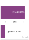
One compressed update is smaller than one raw-data upload; repeated rounds accumulate.

Napkin Math 1.3: Model updates vs. raw data

Problem: A team is designing a federated camera-personalization system that learns from 200 MB of compressed user images per week. Compare one upload of those images with one compressed model-update uplink round.

Math: Bandwidth efficiency is the ratio of raw data volume to model update size.

Raw Data Upload: 200 MB/week.
One Federated Uplink Round: A compressed model update (5M params) is 2.5 MB.
One-Round Uplink Reduction: 200 MB/2.5 MB = 80×.

Systems insight: For this scenario, one 2.5 MB uplink is 80× smaller than one 200 MB raw-data upload. That ratio is not the end-to-end communication saving of a training run: after roughly 80× uplink rounds, cumulative update uploads alone equal the raw-data volume, before counting global-model downloads, retries, or protocol overhead. A deployment must therefore multiply per-round traffic by the expected round count.

The three-phase evolution introduced in 图 3 (local-only, centralized cloud, federated) now resolves into federated learning’s defining position. 图 10 restates that comparison with the emphasis the algorithms section needs: offline learning trains centrally and deploys static models; on-device learning adapts locally but in isolation, sharing no insight across users; and federated learning bridges the two by coordinating updates globally while raw data stays local, so it benefits from distributed model improvements without centralizing the data that produced them.

\begin{tikzpicture}[line join=round,font=\sffamily\small]
\tikzset{
 LineD/.style={line width=0.2pt,black!50,text=black},
 pics/cloud/.style = {
        code = {
\colorlet{red}{BrownLine}
\begin{scope}[local bounding box=CLO,scale=1.8, every node/.append style={transform shape}]
\draw[red,line width=1.25pt,fill=yellow!10](0,0)to[out=170,in=180,distance=11](0.1,0.61)
to[out=90,in=105,distance=17](1.07,0.71)
to[out=20,in=75,distance=7](1.48,0.36)
to[out=350,in=0,distance=7](1.48,0)--(0,0);
\end{scope}
}
},
circles/.pic={
\pgfkeys{/channel/.cd, #1}
\node[circle,draw=\channelcolor,line width=\linewidth,fill=\channelcolor!10,
minimum size=6.5mm](\picname){};
        }
}
\pgfkeys{
  /channel/.cd,
  channelcolor/.store in=\channelcolor,
  drawchannelcolor/.store in=\drawchannelcolor,
  scalefac/.store in=\scalefac,
  linewidth/.store in=\linewidth,
  picname/.store in=\picname,
  channelcolor=BrownLine,
  drawchannelcolor=BrownLine,
  scalefac=1,
  linewidth=0.6pt,
  dashed/.is if=boxdashed,
  dashed/.default=true,
  picname=C
}

\tikzset {
  pics/server/.style = {
    code = {
      \colorlet{red}{BlueLine}
      \begin{scope}[anchor=center, transform shape,scale=0.8, every node/.append style={transform shape}]
        \draw[red,line width=1.25pt,fill=white](-0.55,-0.5) rectangle (0.55,0.5);
\foreach \i in {-0.25,0,0.25} {
                \draw[cyan,line width=1.25pt]( -0.55,\i) -- (0.55, \i);
}
        \foreach \i in {-0.375, -0.125, 0.125, 0.375} {
          \draw[cyan!50!black!90,line width=1.25pt](-0.45,\i)--(0,\i);
          \fill[cyan!50!black!90](0.35,\i) circle (1.5pt);
        }

        \draw[red,line width=1.75pt](0,-0.53) |- (-0.55,-0.7);
        \draw[red,line width=1.75pt](0,-0.53) |- (0.55,-0.7);
      \end{scope}
    }
  }
}

\tikzset {
pics/mobile/.style = {
        code = {
\colorlet{red}{BrownLine}
\begin{scope}[local bounding box=MOB,scale=0.4, every node/.append style={transform shape}]
\node[rectangle,draw=red,minimum height=94,minimum width=57,
            rounded corners=6,thick,fill=red!10](R1){};
\node[rectangle,draw=red,minimum height=67,minimum width=44,thick,fill=white](R2){};
\node[circle,minimum size=8,below= 2pt of R2,inner sep=0pt,thick,fill=red!90]{};
\node[rectangle,fill=red,minimum height=2,minimum width=20,above= 4pt of R2,inner sep=0pt,thick]{};
%
 \end{scope}
     }
  }
}

\newcommand{\mobilni}[1]{
\colorlet{red}{#1}
\begin{scope}[local bounding box=MOB,scale=0.4, every node/.append style={transform shape}]
\node[rectangle,draw=red,minimum height=94,minimum width=57,
            rounded corners=6,thick,fill=red!10](R1){};
\node[rectangle,draw=red,minimum height=67,minimum width=44,thick,fill=white](R2){};
\node[circle,minimum size=8,below= 2pt of R2,inner sep=0pt,thick,fill=red!90]{};
\node[rectangle,fill=red,minimum height=2,minimum width=20,above= 4pt of R2,inner sep=0pt,thick]{};
 \end{scope}
}
\newcommand{\krugovi}[2]{
\begin{scope}[local bounding box=CIRCLE1,shift={($(0,0)+(6.0,0)$)},
scale=#1, every node/.append style={transform shape}]
%1 column
\foreach \j in {1,2} {
  \pgfmathsetmacro{\y}{(1-\j)*0.83 + 0.7}
  \pic at (-2.8,\y) {circles={channelcolor=RedLine, linewidth=#2pt,picname=1CD\j}};
}
%2 column
\foreach \j in {1,2,3} {
  \pgfmathsetmacro{\y}{(1.5-\j)*0.83 + 0.7}
  \pic at (-1.5,\y) {circles={channelcolor=VioletLine, linewidth=#2pt,picname=2CD\j}};
}
%3 column
\foreach \i in {1,...,4} {
  \pgfmathsetmacro{\y}{(2-\i)*0.83+0.7}
  \pic at (0,\y) {circles={channelcolor=BrownLine, linewidth=#2pt,picname=3CD\i}};
}
%4 column
\foreach \j in {1,2,3,4} {
  \pgfmathsetmacro{\y}{(2-\j)*0.83 + 0.7}
  \pic at (1.5,\y) {circles={channelcolor=BlueLine, linewidth=#2pt,picname=4CD\j}};
}
%5 column
\foreach \j in {1,2} {
  \pgfmathsetmacro{\y}{(1-\j)*0.83 + 0.7}
  \pic at (2.8,\y) {circles={channelcolor=RedLine, linewidth=#2pt,picname=5CD\j}};
}
\foreach \i in {1,2}{
  \foreach \j in {1,2,3}{
\draw[LineD](1CD\i)--(2CD\j);
}}
\foreach \i in {1,2,3}{
  \foreach \j in {1,2,3,4}{
\draw[LineD](2CD\i)--(3CD\j);
}}
\foreach \i in {1,2,3,4}{
  \foreach \j in {1,2,3,4}{
\draw[LineD](3CD\i)--(4CD\j);
}}
\foreach \i in {1,2,3,4}{
  \foreach \j in {1,2}{
\draw[LineD](4CD\i)--(5CD\j);
}}
\end{scope}
}

\krugovi{0.6}{0.6}
\node[above=6pt of CIRCLE1](OL){\textbf{Offline learning}};

\begin{scope}[local bounding box=CLOUD1,shift={($(CIRCLE1)+(-1.4,-4.95)$)},
scale=1.2, every node/.append style={transform shape}]
\pic[shift={(0,0)}] at (0,0) {cloud};
\end{scope}

\begin{scope}[local bounding box=SERVER1,shift={($(CLOUD1)+(0,0)$)},
scale=1.2, every node/.append style={transform shape}]
\pic[shift={(-0.1,-0.1)}] at (0,0) {server};
\end{scope}
\node[below=2pt of SERVER1]{Data};
\draw[VioletLine,line width=1pt,-latex,shorten >=2pt,shorten <=-4pt](CLOUD1.80)--(CIRCLE1.288);
\draw[VioletLine,line width=1pt,latex-,shorten >=2pt,shorten <=-4pt](CLOUD1.110)--(CIRCLE1.245);
%%%
%center
\begin{scope}[local bounding box=CENTER]
\begin{scope}[local bounding box=MOBILE1,shift={($(CLOUD1)+(4.5,1.9)$)},
scale=3.35, every node/.append style={transform shape}]
 \pic[shift={(0,0)}] at (0,0) {mobile};
\end{scope}
\begin{scope}[local bounding box=KRUGOVI,shift={($(MOBILE1)+(-6,0)$)},
scale=1, every node/.append style={transform shape}]
\krugovi{0.3}{0.3}
\end{scope}
\node[draw=GreenLine, line width=0.75pt, fill=GreenL!44, align=center,
minimum height=10mm](AM)at($(MOBILE1.east)+(2.5,0)$){Adapt model\\ based on\\ local data};
\draw[VioletLine,line width=1pt,latex-,shorten <=4pt](AM.165)--++(180:1.3);
\draw[VioletLine,line width=1pt,-latex,shorten <=4pt](AM.195)--++(180:1.3);
\end{scope}
\node[below=12pt of CENTER,align=center](LAO){Locally adapt once to a few samples\\ (e.g., few shot learning)
     or continuously\\ (e.g., unsupervised learning)};
%%%%
%RIGHT
\begin{scope}[local bounding box=RIGHT,shift={($(CENTER)+(5.2,0)$)}]
\begin{scope}[local bounding box=CLOUD2,shift={($(0,0)+(0,1.0)$)},
scale=0.65, every node/.append style={transform shape}]
\pic[shift={(0,0)}] at (0,0) {cloud};
\end{scope}
\node[]at(0.8,1.35){Coordinator};

\begin{scope}[local bounding box=MOBILE2,shift={($(CLOUD2)+(-1.25,-2.9)$)},
scale=1.2, every node/.append style={transform shape}]
 \mobilni{OliveLine}
\end{scope}
\begin{scope}[local bounding box=KRUGOVI,shift={($(MOBILE2)+(-3,0)$)},
scale=0.5, every node/.append style={transform shape}]
\krugovi{0.2}{0.2}
\end{scope}
%
\begin{scope}[local bounding box=MOBILE3,shift={($(CLOUD2)+(1.25,-2.9)$)},
scale=1.2, every node/.append style={transform shape}]
 \mobilni{OliveLine}
\end{scope}
\begin{scope}[local bounding box=KRUGOVI,shift={($(MOBILE3)+(-3,0)$)},
scale=0.5, every node/.append style={transform shape}]
\krugovi{0.2}{0.2}
\end{scope}
\node[below=3pt of MOBILE2]{Worker};
\node[below=3pt of MOBILE3]{Worker};
\node[draw=RedLine, line width=0.75pt, fill=RedL!44, align=center,
minimum height=10mm](TD)at($(MOBILE3.east)+(2.25,0)$){Training on \\ local data};
\end{scope}
\node[]at($(MOBILE2)!0.5!(MOBILE3)$){$\bullet$ $\bullet$ $\bullet$};

\draw[VioletLine,line width=1pt,latex-,shorten <=4pt](TD.165)--++(180:1.2);
\draw[VioletLine,line width=1pt,-latex,shorten <=4pt](TD.195)--++(180:1.2);
\draw[VioletLine,line width=1pt,latex-latex,shorten <=1pt](MOBILE2)--
       node[left=4pt,align=center,text=black]{Model \\ updates}(CLOUD2);
       \draw[VioletLine,line width=1pt,latex-latex,shorten <=1pt](MOBILE3)--
       node[right=4pt,align=center,text=black]{5G \\ connectivity}(CLOUD2);
%
\path[red](OL)-|coordinate(MO)(MOBILE1);
\path[red](OL)-|coordinate(CO)(CLOUD2);
\path[red](LAO)-|coordinate(COD)(CLOUD2);
\node[align=center]at($(COD)+(1.5,0)$){Aggregate model updates across \\
multiple users to globally improve\\ model from more diverse data};
\node[]at(MO){\textbf{On-device learning}};
\node[]at(CO){\textbf{Federated learning}};
\end{tikzpicture}

图 10: Federated learning balances data privacy with collective model improvement by coordinating local training across distributed devices, unlike offline learning’s centralized approach or on-device learning’s isolated adaptation. Each paradigm handles data location and model update strategies differently, revealing the trade-offs between personalization, data security, and global knowledge sharing.

Privacy-preserving collaborative learning

Across application domains such as Gboard’s keyboard personalization, wearable health monitoring, and voice interfaces, compact on-device updates solve only the data-movement side of the problem. Federated learning (FL) adds the coordination layer: it trains a shared model across a population of devices without transferring raw data to a central server (McMahan 等 2017年). Unlike traditional centralized training pipelines, which require aggregating all training data in a single location, federated learning distributes the training process itself. Each participating device computes updates based on its local data and contributes to a global model through an aggregation protocol, typically coordinated by a central server.

²⁷ Non-IID Data: Data that is not independently and identically distributed; in data-center training, data shuffling ensures every batch represents the global distribution. On the edge, each user’s data is inherently biased (non-IID): a user in Tokyo mostly types Japanese, while a user in London types English. This bias creates gradient divergence, making standard FedAvg 2–5$\times$ slower to converge than centralized SGD.

This shift aligns closely with mobile, edge, and embedded systems because it preserves data locality while still improving the shared model. However, the privacy and personalization benefits are real only if the system also handles client variability, communication efficiency, and non-i.i.d. data distributions²⁷ through specialized protocols and coordination mechanisms.

Three areas define federated learning in on-device settings: the core learning protocols that govern coordination across devices, strategies for scheduling and communication efficiency, and approaches to personalization. Privacy mechanisms such as secure aggregation and differential privacy wrap these areas rather than replacing them: they determine what the server can infer from updates and how much noise the training loop must absorb.

The first architectural decision is whether the participants form a cross-device or cross-silo federation. The distinction changes the failure model, scheduling policy, and privacy unit before any optimizer is selected (Kairouz 和 McMahan 2021年). 表 4 makes those consequences explicit.

表 4: Cross-Device and Cross-Silo Federated Learning: The participant population determines scheduling, trust, weighting, and privacy semantics. A protocol designed for millions of unreliable phones is not automatically appropriate for a consortium of hospitals.

Design dimension	Cross-device federation	Cross-silo federation
Participants	Large population of intermittently available personal devices	Small set of known organizations or sites
Round semantics	Sample an eligible cohort; expect stragglers and dropouts	Coordinate a stable membership; investigate missing sites
Trust boundary	Treat client software and local data as potentially compromised	Authenticate institutions, but still isolate each data custodian
Weighting default	Decide whether the objective represents examples or users	Weighting follows the agreed institutional objective, not site size by default
Privacy unit	Usually a user or device across its participation history	Usually a person or record within a site’s data, sometimes the site itself

Learning protocols

The protocols that make distributed coordination practical at scale must solve three engineering challenges simultaneously: ensuring that local training produces compatible updates despite non-IID data distributions, aggregating those updates efficiently despite bandwidth constraints, and coordinating timing across devices with heterogeneous availability patterns.

Local training

Local training is the point where privacy preservation becomes a systems boundary. Individual devices compute model updates from private data, but every local choice affects the validity of the aggregate: which base model the device starts from, which local examples it samples, how much optimization it performs, and what update it sends back. The loop is therefore useful to present as an ordered protocol rather than as an abstract definition:

Model Initialization: Each device initializes its local model parameters, often by downloading the latest global model from the server.
Local Data Sampling: The device samples a subset of its local data for training. This data may be non-IID, meaning that it may not be uniformly distributed across devices.
Local Training: The device performs a number of training iterations on its local data, updating the model parameters based on the computed gradients.
Model Update: After local training, the device computes a model update (e.g., the difference between the updated and initial parameters) and prepares to send it to the server.
Communication: The device transmits the model update to the server, typically using a secure communication channel to protect user privacy.
Model Aggregation: The server aggregates the updates from multiple devices to produce a new global model, which is then distributed back to the participating devices.

The process repeats iteratively, with devices periodically downloading the latest global model and performing local training. Update frequency varies based on system constraints, device availability, and communication costs.

Federated aggregation protocols

The central coordination mechanism in federated learning allows devices with small, local datasets to collaboratively train a shared model. Client devices perform local training and transmit model updates to a central server, which aggregates them into a refined global model and redistributes it for the next training round. The cyclical procedure decouples learning from centralized data collection, suiting environments where user data is private, bandwidth is constrained, and device participation is sporadic.

The most widely used baseline for this process is federated averaging (FedAvg),²⁸ which has become a canonical algorithm for federated learning (McMahan 等 2017年). In FedAvg, each device trains its local copy of the model using SGD on its private data.

²⁸ FedAvg (Federated Averaging): McMahan 等 (2017年) average model weights instead of individual gradients, allowing each client to perform multiple local SGD steps (typically 1–20) before a single upload. This reduces communication by 10–100$\times$ compared to distributed SGD, making federated learning viable over mobile networks where upload bandwidth is the binding constraint. The trade-off: more local steps improve communication efficiency but increase divergence on non-IID data, requiring careful tuning per deployment.

McMahan, Brendan, Eider Moore, Daniel Ramage, Seth Hampson, 和 Blaise Agüera y Arcas. 2017年. 《Communication-Efficient Learning of Deep Networks from Decentralized Data》. International Conference on Artificial Intelligence and Statistics (AISTATS), Proceedings of Machine Learning Research, 卷 54: 1273～82.

Formally, let $\mathcal{D}_k$ denote the local dataset on client $k$, and let $\theta_k^t$ be the parameters of the model on client $k$ at round $t$. Each client performs $E$ epochs of SGD on its local data, yielding an update $\theta_k^{t+1}$. The central server then aggregates these updates as: \[ \theta^{t+1} = \sum_{k=1}^{C} \frac{n_k}{n} \theta_k^{t+1} \tag{2}\] 其中，$n_k = |\mathcal{D}_k|$ 表示设备 $k$ 上的样本数，$n = \sum_k n_k$ 表示参与客户端的样本总数，$C$ 表示当前轮次中的活跃设备数。

该公式优化的是一个示例加权目标：本地示例数多一倍的客户端获得一倍的权重影响。当每个示例都应同等贡献时，这一选择是恰当的；但它可能让 prolific users 或大型机构主导模型。改为用户加权目标后，每个参与客户端的权重为 $1/C$，可在聚合前对每个客户端的本地贡献进行截断或归一化。两种选择都不具有普适的公平性。系统必须声明其兴趣单元是示例、用户、组织还是部署队列，然后评估该人群，而不是把 $n_k/n$ 当作实现默认值继承下来。

缓解慢节点

在由数百万台异构设备组成的集群中，等待每个被选中的客户端都上报其更新并不现实。网络延迟、电池耗尽或后台进程争用都可能导致某些设备（“慢节点” stragglers）比平均情况慢 10$\times$。在轮次语义层面，后果是直接的：公式 2 中的加权聚合必须等待足够多的更新才能进行，因此轮次时长由服务器仍在等待的最慢设备决定。针对这一问题的调度对策是超选（over-selection），它是一种客户端调度策略，并与客户端调度的其余部分一起在节 1.5.1 中展开。

该循环式协调协议构成了联邦学习的基础。图 11 将 Federated Averaging 协议分解为四个阶段：客户端选择（通过超选处理慢节点）、在私有数据上进行本地训练、带可选压缩的参数上传，以及加权聚合以生成更新后的全局模型。

图 11: 联邦平均协议：四阶段循环始于服务器向参与客户端广播全局模型。客户端在私有数据上进行本地训练并上传模型更新，服务器将这些更新聚合为下一个全局模型。

这一基本结构引入了若干设计选择与权衡。本地轮次数量 $E$ 会影响计算与通信之间的平衡：更大的 $E$ 可以降低通信频率，但若本地数据分布差异过大，则可能带来发散风险。参与客户端的选择会影响收敛稳定性与公平性。在实际部署中，并非所有设备都随时可用，硬件能力也可能存在显著差异，因而需要鲁棒的参与调度与故障容错机制。

联邦学习收敛性分析

联邦学习是否能够收敛、以及达到可接受精度所需的速度有多快，是系统设计中的关键问题。与集中式训练（其收敛性主要取决于学习率和批大小）不同，联邦学习的收敛性取决于通信轮次、本地计算、客户端参与和数据异构性之间的相互作用。这些因素决定了联邦部署能否在数小时、数天内达到目标精度，或者根本达不到。 集群规模弱扩展 提出了弱扩展性论证，说明为何增加参与设备数量会使总工作量增长快于墙钟时间的减少，从而界定此处客户端参与能够加速收敛的上限。

收敛速率基础

一种有用的系统抽象是同时跟踪参与客户端、本地轮次和通信轮次。 McMahan 等 (2017年) 用这些控制量来定义 FedAvg，但它们并不能仅凭其乘积确立普适的收敛速率。为说明这些控制量可能朝相反方向发挥作用，本章采用如下无量纲玩具敏感度分数：

\[ S_{\text{toy}}(C,E,R;\beta_{\text{het}}) = \frac{\sigma(1+\beta_{\text{het}})}{\sqrt{CER}} + \frac{\beta_{\text{het}}^2 E^2}{R} \]

此处，$C$ 表示每轮参与客户端的数量，$E$ 表示本地轮次（本地 epoch）的数量，$R$ 表示通信轮次的数量，$\sigma$ 是无量纲的场景常数，$\beta_{\text{het}}$ 是无量纲的客户端漂移旋钮。第一项会随着处理的客户端—epoch 数量增加而下降，而第二项则刻意对异质性下较大的 $E$ 施加惩罚。该分数既不是收敛定理，也不是经验校准的估计器，更不是目标差距的预测器。

乘积 $CER$ 仅可作为客户端—epoch 计数的记账工具。$CER$ 相等并不意味着收敛程度相同，因为客户端采样、每个客户端的样本数、批大小、步长、本地更新漂移以及数据分布都可能不同。因此，生产环境中的选择需要借助测量，或采用假设与所部署的优化器及数据相匹配的收敛性结果。

非独立同分布（Non-IID）数据对的影响

联邦学习综述与实证研究将非独立同分布数据视为核心收敛挑战，并采用诸如局部不相似性、地球移动者距离（earth mover’s distance）或权重发散等度量 Zhao 等 (2018年)。这些度量之间不可互换。在玩具分数中，$\beta_{\text{het}}$ 仅是一个场景旋钮：将其设为零即可移除漂移项，而增大它则会使额外的本地 epoch 更加昂贵。它并不具有普适的量纲，也不存在跨应用的直接估计器。

$E^2/R$ 项编码了一种定性交互：更多的本地工作可以降低通信频率，但也可能在目标不一致时增加客户端漂移。指数与系数是本次敏感性分析的假设，而非对每一个 FedAvg 部署的论断。

玩具异质性敏感性示例

由于 $\beta_{\text{het}}$ 并非实测指标，不应按应用领域赋予其经验取值范围。下方算例仅选取 $\beta_{\text{het}}=1.5$，用以展示玩具分数的算术过程；该取值并不能刻画键盘、语言或健康数据。

一个假设性配置，包含 100 个客户端，使这个玩具算例具体化：每轮选取 $C$ = 10 个客户端，每轮本地轮次 $E$ = 5，各分量分数阈值 $\epsilon$ = 0.01，以及两种场景设定，$\beta_{\text{het}}$ = 0 和 $\beta_{\text{het}}$ = 1.5。这些输入并不描述生产部署。

零漂移玩具算例 $(\beta_{\text{het}} = 0)$：令第二个分量为零，场景选择为 $\sigma=1$，将第一个分量设为不超过 $\epsilon$，可得：

\[ R_{\text{IID}} \geq \frac{\sigma^2}{C \cdot E \cdot \epsilon^2} = \frac{1}{10 \cdot 5 \cdot 0.0001} = 200 \text{ rounds} \]

每轮有 10 个客户端、每个客户端本地训练 5 个轮次，这代表 200 $\times$ 10 $\times$ 5 = 10,000 的总客户端轮次计算量。

正漂移玩具案例 $(\beta_{\text{het}} = 1.5)$：分别对两个分量应用阈值。在 $E=5$ 下，第一个分量需要 1,250 轮，而假设的漂移分量需要：

\[ \frac{\beta_{\text{het}}^2 E^2}{R} \leq \epsilon \implies R \geq \frac{\beta_{\text{het}}^2 E^2}{\epsilon} = \frac{2.25 \times 25}{0.01} = 5,625 \text{ rounds} \]

更大的组件阈值比零漂移场景高约 28.1×。它对应 5,625 $\times$ 10 $\times$ 5 = 281,250 轮客户端轮次。这些是所选玩具常数的输出，而非预测的收敛成本。

假设的 $E^2$ 漂移项使分数对本地轮次选择敏感。若使用 $E = 2$ 而非 $E = 5$，漂移分量阈值缩小至 900 轮，而第一分量阈值增大至 3,125：

\[ R \geq \max\left(\frac{(1+\beta_{\text{het}})^2}{C \cdot E \cdot \epsilon^2}, \frac{\beta_{\text{het}}^2 E^2}{\epsilon}\right) = \max\left(\frac{2.5^2}{10 \cdot 2 \cdot 0.0001}, \frac{2.25 \times 4}{0.01}\right) = \max(3,125, 900) = 3,125 \text{ rounds} \]

在本玩具评分中，跨阈值的轮次数量下降 1.80×，而每轮本地工作下降 2.5×。客户端轮次数量变为 3,125 $\times$ 10 $\times$ 2 = 62,500，即相对 4.5× = $E$ 场景的 5 倍减少。这仅展示了所假设公式所编码的敏感性；实际部署必须通过经验估计该权衡，或采用适用的收敛性结果。

通信—计算权衡

本地轮次与通信轮次之间的相互作用构成了一个根本性的设计权衡，如图图 12 所示。更多的本地轮次会降低通信频率（计算方面的收益），但会增加客户端漂移（统计方面的代价）；而更少的本地轮次则能保持更紧密的同步，但通信成本更高。

\begin{tikzpicture}[font=\small\sffamily, scale=0.85, node distance=1cm and 1cm]
  \tikzset{
    Axis/.style={->, line width=0.75pt},
    CurveIID/.style={BlueLine, line width=1.0pt},
    CurveNonIID/.style={RedLine, line width=1.0pt},
    Annot/.style={dashed, BrownLine, line width=1.0pt},
    Label/.style={font=\tiny\sffamily}
  }

  % Axes
  \node (origin) at (0,0) {};
  \draw[Axis] (origin) -- ++(8,0) node[right] {Local Epochs $E$};
  \draw[Axis] (origin) -- ++(0,5) node[above] {Rounds to $\epsilon$-optimal};

  % IID curve (nearly flat)
  \begin{scope}[shift={(origin)}]
    \draw[CurveIID] plot[smooth] coordinates {(0.5,1.2) (2,1.0) (4,0.9) (6,0.85) (7.5,0.82)};
    \node[BlueLine, right] at (7.5,1.2) {IID ($\beta_{\text{het}}=0$)};
  \end{scope}

  % Non-IID curve (quadratic growth)
  \begin{scope}[shift={(origin)}]
    \draw[CurveNonIID] plot[smooth] coordinates {(0.5,0.8) (2,1.5) (4,3.2) (6,4.5) (7,4.8)};
    \node[RedLine, right] at (5.5,4.8) {Non-IID ($\beta_{\text{het}}=1.5$)};
  \end{scope}

  % Optimal region annotation
  \begin{scope}[shift={(origin)}]
    \draw[Annot] (2,0) -- (2,1.5);
    \node[Label, below] at (2,0) {Sweet spot};
    \node[Label, align=center] at (4,2.2) {Client drift\\dominates};
  \end{scope}

  % Axis labels
  \node[Label, below=of origin, xshift=1cm] {1};
  \node[Label, below=of origin, xshift=4cm] {5};
  \node[Label, below=of origin, xshift=7cm] {10};
  \node[Label, left=of origin, yshift=1cm] {100};
  \node[Label, left=of origin, yshift=2.5cm] {500};
  \node[Label, left=of origin, yshift=4cm] {1000};
\end{tikzpicture}

图 12: 通信—计算权衡：该示意图展示了在数据非独立同分布（non-IID）条件下，每轮执行更多本地工作与累积客户端漂移之间的定性张力。其 $\epsilon$-optimal 轴和运行点标签均为示意性简写，并非收敛性保证，也不构成普适的最优轮次数范围；系统设计者必须测量所部署的优化器、数据和客户端群体。

最优运行点取决于部署特定的因素。通信成本（带宽、能耗）倾向于更大的 $E$，而在异构性下的收敛速度则倾向于更小的 $E$。实际系统常采用自适应策略：从较小的 $E$ 起步，随着模型接近收敛、客户端漂移减弱而逐步增大。

当联邦学习在下运行时

联邦学习只有在若干部署条件有利时才能实现实际收敛，这一主题在联邦学习系统的综述与开放问题中得到了强调 (Kairouz 和 McMahan 2021年)：

异构性必须受到足够约束，使得客户端漂移不会主导训练时间。当人群高度异构时，将客户端聚类为更同质的组，或采用个性化方法，可能优于单一全局模型。
客户端参与率必须足够高，以提供稳定的聚合更新。极低的参与率会使梯度估计产生噪声，并加剧选择偏差。
每个参与客户端都需要足够的本地数据以完成有意义的更新计算。极小的本地批次可能贡献高方差更新，从而 destabilize 训练。

当这些条件被违反时，就必须采用替代方法。严重的异构性提示采用分层联邦学习，进行区域级聚合，或采用无需全局聚合的完全个性化模型。极低的参与率表明需要异步协议，即不要求同步轮次。本地数据极少的客户端则受益于小样本自适应技术，而非基于梯度的训练。

这些数学聚合协议证明了去中心化学习在理论上是可行的。在实验室中，在十个可靠节点上执行联邦平均是轻而易举的；而在一千万部频繁进出蜂窝网络的智能手机上执行它，则是另一个工程问题。稳健的联邦系统必须将算法转化为编排、调度与故障处理机制，并且从一开始就假定客户端不可靠。

联邦学习：规模化系统

在教科书式的算法中，全部 100 个边缘设备都完美地计算出自己的更新，并在完全相同的时间点向服务器报告。而在现实中，跨越一百万部智能手机的联邦学习轮次必须处理设备过热、失去 Wi-Fi、进入省电模式或关机等情况。在规模化条件下构建联邦系统，意味着要工程化一个能够容忍异步掉线与极端慢节点（stragglers）作为标准运行条件的编排器。

客户端调度

联邦学习建立在这样一个假设之上：客户端，即持有本地数据的设备，会周期性地变得可用于参与训练轮次。在真实系统中，客户端可用性是间歇且多变的。设备可能在任何给定时刻处于关机、断电、缺乏网络访问，或以其他方式无法参与的状态。因此，客户端调度在分布式学习的有效性与效率中居于核心地位。

在基础层面，联邦机器学习系统会定义参与的资格标准。设备必须满足最低要求，例如处于插电状态、连接 Wi-Fi、处于空闲状态，以避免干扰用户体验或耗尽电池资源。这些标准决定了总体人群中哪个子集在每一轮训练中被视为“可用”。

除了这些运行层面的过滤条件，设备在硬件能力、数据可用性与网络条件方面也存在差异。有些智能手机包含大量与当前任务相关的近期样本，而另一些则只有过时或无关的数据。网络带宽与上传速度可能因地理位置与运营商基础设施而差异很大。因此，随机选择客户端可能导致对底层数据分布覆盖不足，以及模型收敛不稳定。

基于可用性的选择会引入参与偏差。具备有利条件的客户端更有可能反复参与。这些有利条件包括频繁充电、高端硬件以及稳定的连接。与此同时，其他设备则被系统性地下代表不足。这会使最终模型偏向于某个特权子集的行为与偏好，从而引发公平性与泛化方面的担忧。

参与偏差的严重性在考察真实部署统计时便显现出来。关于联邦学习部署的研究表明，最活跃的 10% 设备可以贡献超过 50% 的训练轮次，而排名靠后的 50% 设备可能从头到尾都不参与。这形成了一个反馈回路：模型被针对拥有高端设备且连接稳定的用户优化得更加彻底，从而可能损害最需要自适应的资源受限用户的表现。一个键盘预测模型可能偏向于那些整夜充电的旗舰手机用户的输入模式，而遗漏了来自预算设备用户或不规律充电用户的重要语言差异。

为应对这些挑战，系统必须在调度效率与客户端多样性之间取得平衡。一种关键方法采用分层或配额式采样，以确保不同群体中的客户端参与具有代表性。一些系统实现了“公平预算”，用于跟踪累计参与情况，并在相关设备变得可用时主动优先处理代表性不足的客户端。另一些系统则采用重要性采样技术，依据估计的人群统计而非原始参与率来重新加权贡献。例如，基于异步缓冲的技术允许参与客户端独立地贡献模型更新，而无需在每一轮中同步协调 (Nguyen 等 2021年)。该模型已被扩展以纳入新鲜度感知 (Rodio 和 Neglia 2024年) 与公平性机制 (Ma 等 2024年)，从而防止过度活跃的客户端主导训练过程。

Nguyen, John, Kshitiz Malik, Hongyuan Zhan, Ashkan Yousefpour, Michael Rabbat, Mani Malek, 和 Dzmitry Huba. 2021年. 《Federated Learning with Buffered Asynchronous Aggregation》. Proceedings of Machine Learning Research (AISTATS) 164.

Rodio, Angelo, 和 Giovanni Neglia. 2024年. 《FedStale: leveraging stale client updates in federated learning》. Frontiers in Artificial Intelligence and Applications (ECAI 2024) 78. https://doi.org/10.3233/faia240849.

Ma, Jeffrey, Alan Tu, Yiling Chen, 和 Vijay Janapa Reddi. 2024年. 《FedStaleWeight: Buffered Asynchronous Federated Learning with Fair Aggregation via Staleness Reweighting》. arXiv preprint arXiv:2406.02877.

这些公平性机制与自适应客户端选择策略并行存在。联邦机器学习系统可以优先选择代表性数据不足的客户端，针对较少被采样的地理区域或人口统计群体，并利用历史参与数据来强制公平性约束。预测建模可以预判客户端后续的可用性或成功率，从而提高训练吞吐量。

被选中的客户端在其私有数据上执行一个或多个本地训练步骤，并将模型更新传输给中央服务器。这些更新会被聚合以形成新的全局模型。通常，这种聚合是加权的，即在平均之前将每个客户端的贡献按一定比例缩放，例如按训练期间使用的本地样本数量。这确保了拥有更具代表性或更大规模数据集的客户端对全局模型施加成比例的权重影响。

调度还必须为轮次等待最慢参与者的时间设定上限。正如节 1.4.2.3 中所确立的，慢节点可能比中位设备慢 10$\times$ 倍，而轮次在收到足够更新之前无法完成聚合。

过选策略在首个 K 个更新到达时结束轮次。

为防止全局模型更新停滞，生产级联邦学习系统采用过选策略。服务器选取的候选池规模 $K_{\text{candidates}}$ 大于目标更新数量 $K_{\text{target}}$（通常为 $K_{\text{candidates}} \approx 1.3 \times K_{\text{target}}$）。服务器聚合前 $K_{\text{target}}$ 个响应者的更新并丢弃其余部分。该方法将轮次时长限定为第 $K_{\text{target}}$ 快设备的速度，而非绝对最慢设备，从而大幅缩短收敛的墙钟时间。

这些调度决策直接影响收敛速率、模型泛化能力、能耗以及整体用户体验。调度不佳会导致拖慢者过多、对狭窄的客户端群体过拟合，或产生无效计算。因此，客户端调度是联邦学习系统设计的核心组成部分，既需要算法层面的洞察，也需要基础设施层面的协同。

Checkpoint 1.3: 联邦系统设计

设想为 1000 万部移动设备构建一个联邦学习系统。数据高度非独立同分布（用户具有各自成簇的打字模式），网络环境受限（1–10 Mbps）。在选择该场景的优化方案之前，先分类本地瓶颈，并说明每个决策由哪项系统约束主导。

考虑三项设计决策：

聚合：为非独立同分布群体选择朴素 FedAvg、减少本地轮次，还是个性化/聚类，并说明该选择如何控制客户端漂移。
隐私：判断该部署是否需要正式的差分隐私噪声，还是安全聚合与数据最小化已足以应对所述威胁模型；定性说明预期的收敛时间成本。
通信：在受限带宽下，选择梯度量化（例如 8-bit）还是结构化稀疏，并论证带宽/精度之间的权衡。

带宽感知的更新压缩

更新压缩首先是一种瓶颈诊断，其次才是一项技术选择：如果每个轮次都传输完整的模型权重或梯度，那么移动带宽和电池预算会在优化器发挥作用之前决定收敛。²⁹ 设计决策在于：哪些信息可以量化、稀疏化，或保留在本地，同时仍能保持足够的梯度保真度以使 FedAvg 收敛。

²⁹ 无线上传非对称性：LTE 上传平均为 5–10 Mbps，而下载为 50+ Mbps，由此形成主导联邦学习设计的非对称瓶颈；传输 50 MB 的模型更新约消耗 100 mAh（2–3% 的电量），在 LTE 下耗时 40–80 秒。低功耗协议更差：LoRaWAN 最高仅 50 kbps，占空比为 1%，使得未压缩的更新在物理上不可行。这种非对称性正是梯度压缩并非可选项、而是架构必需的原因。

³⁰ 梯度量化：在传输前将 FP32 梯度转换为更低精度（INT8、INT4 或 1-bit）。量化 SGD 与 signSGD 等技术表明，量化或仅符号更新可大幅降低通信开销，同时依靠随机量化或误差补偿来保持收敛行为 Bernstein 等 (2018年)。实际获得的字节减少量与精度影响取决于优化器、模型、数据异质性以及残差处理方式。

Bernstein, Jeremy, Yu-Xiang Wang, Kamyar Azizzadenesheli, 和 Animashree Anandkumar. 2018年. 《signSGD: Compressed Optimisation for Non-Convex Problems》. International Conference on Machine Learning (ICML) 80: 560～69.

³¹ 梯度稀疏化：仅按幅度传输幅度最高的 1–10% 的梯度，利用“大多数梯度元素接近零、对收敛贡献甚微”这一观察。本地梯度累加将未传输的残差存储起来，直到其增长到足够大才发送，从而实现 10–100$\times$ 倍的压缩，同时保持训练质量，这一模式被稀疏化 SGD 与深度梯度压缩所采用 Lin 等 (2018年)。权衡之处：过于激进的稀疏化可能使更新偏向频繁激活的参数，从而降低对罕见用户模式的个性化能力。

Lin, Yujun, Song Han, Huizi Mao, Yu Wang, 和 William J Dally. 2018年. 《Deep gradient compression: Reducing the communication bandwidth for distributed training》. International Conference on Learning Representations (ICLR).

压缩决策可分解为三个杠杆，每个杠杆改变通信瓶颈的不同部分：模型压缩降低每次更新的比特数，选择性共享减少传输的参数范围，架构划分则将部分状态保留在本地。模型压缩方法旨在通过量化³⁰、稀疏化或子采样来减小所传输更新的大小，图 14 对此进行了说明。客户端不再发送全精度梯度，而是传输 8-bit 量化更新，或仅通信幅度最高的前 $k$ 个梯度元素³¹。这些变换属于通信机制，而非隐私机制；较小的嵌入、稀疏更新或低精度梯度仍可能泄露成员信息、属性或可重构特征。

选择性更新共享进一步降低通信开销，仅传输模型参数或更新的子集。在分层选择性共享中，客户端仅更新某些层（通常是最终分类器或适配器模块），而将主干部分的多数层保持冻结。这既降低了上传成本，也降低了对共享表示过拟合到非代表性客户端数据的风险。

拆分模型与架构划分将模型划分为共享的全局组件与本地组件。客户端独立训练和维护本地模块，仅与服务器同步共享部分。这降低了通信开销并缩小了暴露范围，但共享更新仍可能泄露信息；隐私主张取决于威胁模型，以及安全聚合或差分隐私等控制手段。

上述方法均在 FedAvg 聚合协议（节 1.4.2.2）之内运行：压缩改变的是每个客户端传输的内容，而非服务器如何组合更新。轮次 $r$ 的完整通信账目为

\[ B_r = B_{\text{download},r} + B_{\text{upload},r} + B_{\text{protocol},r} + B_{\text{retry},r}, \tag{3}\]

公式 3 makes download, upload, protocol, and retry traffic explicit. The download distributes model state, the upload carries client updates, protocol traffic covers authentication and cryptographic setup, and retries account for failed or repeated transfers. Optimizing only $B_{\text{upload},r}$ can therefore move rather than remove the bottleneck. While 图 13 illustrates the trade-off between local computation and network bandwidth, other communication-efficient updates introduce their own costs. Compression may degrade gradient fidelity, selective updates can limit model capacity, and split architectures may complicate coordination. Effective federated learning requires balancing communication, privacy, and convergence against the capabilities and variability of the client population. 压缩的成本效益 works the compression break-even threshold through a worked example.

Unlike the qualitative convergence schematic in 图 12, 图 13 models end-to-end training time under three illustrative network regimes. It makes communication latency part of the objective rather than treating round count alone as the proxy.

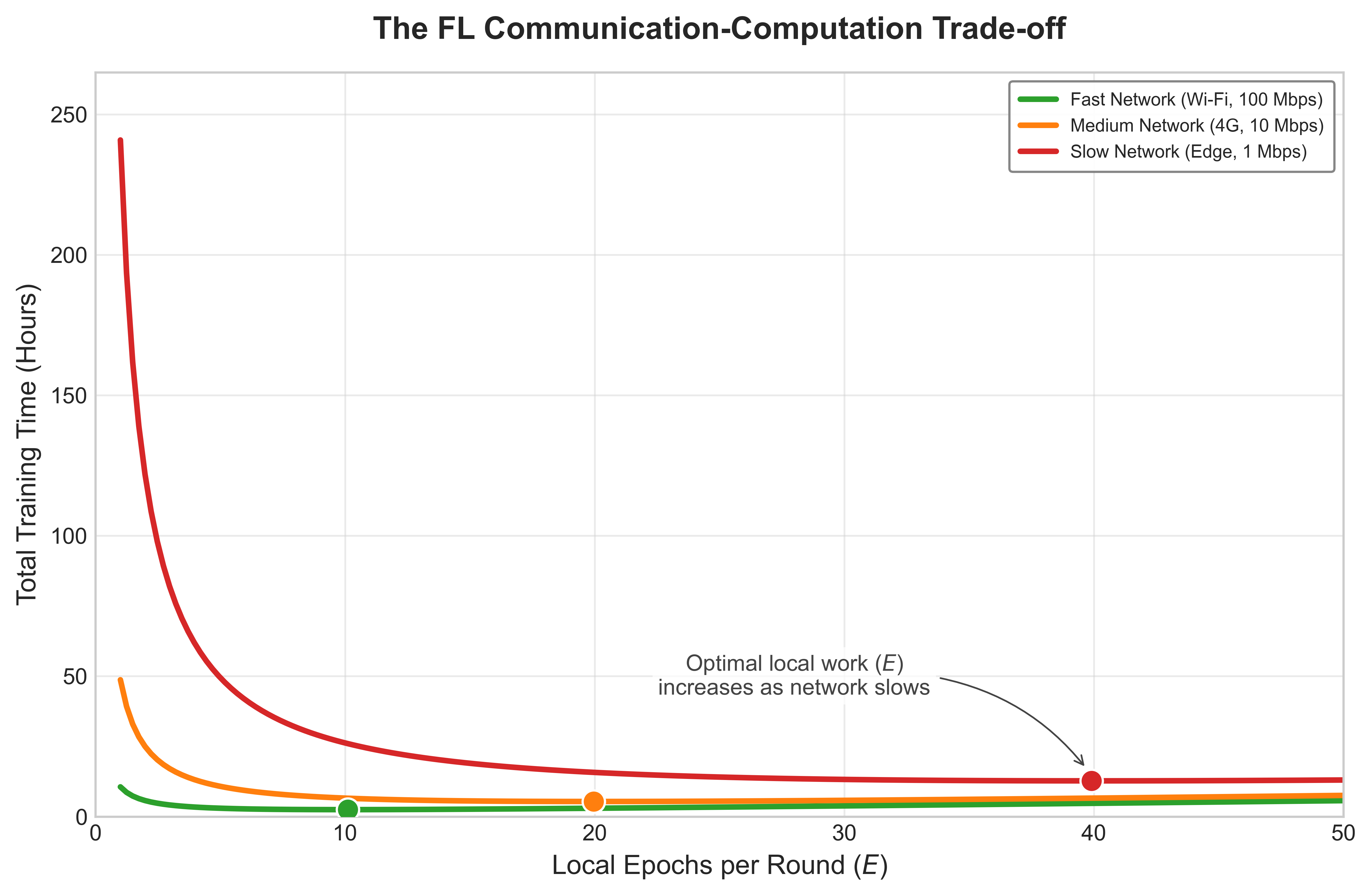
图 13: **Communication-computation trade-off in federated learning**: As network bandwidth decreases from fast to slow, the time-minimizing number of local epochs shifts rightward because additional local computation amortizes more communication. Excessive local work eventually increases total time when client drift requires more global rounds to converge.

Once the system chooses how much local work to perform, update compression determines how much each round must transmit.

\begin{tikzpicture}[font=\small\sffamily, node distance=0pt]
  \tikzset{
    Box/.style={draw=BlueLine, line width=0.75pt, minimum width=0.8cm, minimum height=0.8cm, font=\tiny\sffamily, fill=BlueL, outer sep=0pt},
    BoxOrange/.style={Box, draw=OrangeLine, fill=OrangeL},
    BoxGreen/.style={Box, draw=GreenLine, fill=GreenL},
    Line/.style={->, line width=1.0pt, BlueLine},
    Title/.style={font=\bfseries\sffamily\bfseries, align=center, anchor=south},
    Sub/.style={font=\tiny\sffamily, align=center, anchor=north}
  }

  \begin{scope}[local bounding box=std]
    \node[Box] (s1) {0.5};
    \node[Box, right=of s1] (s2) {-0.2};
    \node[Box, right=of s2] (s3) {0.01};
    \node[Box, right=of s3] (s4) {0.8};
    \node[Title, above=0.2cm of s2.north east] {\textbf{(a) Standard}};
    \node[Sub, below=0.1cm of s2.south east] {FP32: 128 bits};
  \end{scope}

  \begin{scope}[local bounding box=quant]
    \node[BoxOrange, right=1.5cm of std] (q1) {+1};
    \node[BoxOrange, right=of q1] (q2) {0};
    \node[BoxOrange, right=of q2] (q3) {0};
    \node[BoxOrange, right=of q3] (q4) {+2};
    \node[Title, above=0.2cm of q2.north east] {\textbf{(b) Quantization}};
    \node[Sub, below=0.1cm of q2.south east] {INT8: 32 bits (4$\times$)};
  \end{scope}

  \begin{scope}[local bounding box=sparse]
    \node[BoxGreen, right=1.5cm of quant] (sp1) {0.5};
    \node[BoxGreen, right=of sp1] (sp2) {-};
    \node[BoxGreen, right=of sp2] (sp3) {-};
    \node[BoxGreen, right=of sp3] (sp4) {0.8};
    \node[Title, above=0.2cm of sp2.north east] {\textbf{(c) Sparsification}};
    \node[Sub, below=0.1cm of sp2.south east] {Top-k FP32: $\geq$64 bits + idx ($\leq$2$\times$)};
  \end{scope}

  \node[draw=BlueLine, dashed, rounded corners=2pt, line width=0.75pt, minimum width=10cm, minimum height=1cm, below=1.5cm of quant] (server) {Federated Aggregator (Server)};

  \draw[Line] (std.south) -- (std.south |- server.north) node[midway, right, font=\tiny\sffamily, text=black] {Network Transfer};
  \draw[Line] (quant.south) -- (server.north);
  \draw[Line] (sparse.south) -- (sparse.south |- server.north);

\end{tikzpicture}

图 14: Gradient compression techniques: Standard updates transmit full-precision values; quantization maps values to lower-precision buckets, such as FP32 to INT8; and sparsification transmits only the most significant top-$k$ gradients. The latter two mechanisms reduce bytes transferred but introduce representation error or residual state that the training algorithm must manage.

These compression techniques collectively shrink the update payload, ensuring federated rounds remain viable even over severely constrained mobile networks.

Federated personalization

While compression and communication strategies improve scalability, they do not address an important limitation of the global federated learning paradigm, its inability to capture user-specific variation. In real-world deployments, devices often observe distinct and heterogeneous data distributions. A one-size-fits-all global model may underperform when applied uniformly across diverse users. This motivates the need for personalized federated learning, where local models are adapted to user-specific data without compromising the benefits of global coordination.

Let $\theta_k$ denote the model parameters on client $k$, and $\theta_{\text{global}}$ the aggregated global model. For $K$ clients, traditional FL seeks to minimize a global objective: \[ \min_\theta \sum_{k=1}^K w_k \mathcal{L}_k(\theta) \] where $\mathcal{L}_k(\theta)$ is the local loss on client $k$, and $w_k$ is a weighting factor (e.g., proportional to local dataset size). However, this formulation assumes that a single model $\theta$ can serve all users well. In practice, local loss landscapes $\mathcal{L}_k$ often differ significantly across clients, reflecting non-IID data distributions and varying task requirements.

Personalization modifies this objective to allow each client to maintain its own adapted parameters $\theta_k$, optimized with respect to both the global model and local data: \[ \min_{\theta_1, \ldots, \theta_K} \sum_{k=1}^K \left( \mathcal{L}_k(\theta_k) + \lambda_{\text{reg}} \cdot \mathcal{R}(\theta_k, \theta_{\text{global}}) \right) \]

Here, $\mathcal{R}$ is a regularization term that penalizes deviation from the global model, and $\lambda_{\text{reg}}$ controls the strength of this penalty. This formulation allows local models to deviate as needed, while still benefiting from global coordination.

Real-world use cases illustrate the importance of this approach. Consider a wearable health monitor that tracks physiological signals to classify physical activities. While a global model may perform reasonably well across the population, individual users exhibit unique motion patterns, gait signatures, or sensor placements. Personalized finetuning of the final classification layer or low-rank adapters allows improved accuracy, particularly for rare or user-specific classes.

Several personalization strategies address the trade-offs between compute overhead, information exposure, and adaptation speed. One widely used approach is local finetuning, in which each client downloads the latest global model and performs a small number of gradient steps using its local data. This method avoids transmitting those examples during adaptation, but the resulting local state and any later update remain privacy-sensitive. It may also yield suboptimal results when the global model is poorly aligned with the client’s data distribution or when the local dataset is extremely limited.

Another effective technique involves personalization layers, where the model is partitioned into a shared backbone and a lightweight, client-specific head, typically the final classification layer (Arivazhagan 等 2019年). Only the head is updated on-device, reducing memory usage and training time. This approach is particularly well-suited for scenarios in which the primary variation across clients lies in output categories or decision boundaries.

Arivazhagan, Manoj Ghuhan, Vinay Aggarwal, Aaditya Kumar Singh, 和 Sunav Choudhary. 2019年. 《Federated Learning with Personalization Layers》. CoRR abs/1912.00818.

Clustered federated learning offers an alternative by grouping clients according to similarities in their data or performance characteristics, and training separate models for each cluster. This strategy can enhance accuracy within homogeneous subpopulations but introduces additional system complexity and may require exchanging metadata to determine group membership.

Finally, meta-learning approaches, such as model-agnostic meta-learning (MAML),³² aim to produce a global model initialization that can be quickly adapted to new tasks with just a few local updates (Finn 等 2017年). This technique is especially useful when clients have limited data or operate in environments with frequent distributional shifts.

³² MAML (Model-Agnostic Meta-Learning): Finn 等 (2017年) optimize for a model initialization from which one or a few gradient steps can yield good performance on a new task, with experiments including one-shot and few-shot settings. Meta-training is more expensive than ordinary finetuning because it differentiates through the adaptation process, but deployment adaptation can be limited to a small number of local updates. This makes MAML relevant for edge scenarios where inference compute is cheap but training data is scarce.

Finn, Chelsea, Pieter Abbeel, 和 Sergey Levine. 2017年. 《Model-agnostic meta-learning for fast adaptation of deep networks》. Proceedings of the 34th International Conference on Machine Learning (ICML).

Each of these strategies reflects a different point in the personalization trade-off space. Examine 表 5 to see how compute overhead, privacy guarantees, and adaptation latency vary across local finetuning, personalization layers, clustered federated learning, and meta-learning approaches.

表 5: Personalization Trade-Offs: Federated learning strategies balance personalization with compute, information exposure, and adaptation latency. Data locality narrows exposure but does not by itself provide a privacy guarantee.

Strategy	Personalization Mechanism	Compute Overhead	Privacy Preservation	Adaptation Speed
Local Finetuning	Gradient descent on local loss postaggregation	Low to Moderate	Raw examples stay local; adapted state remains sensitive	Fast (few steps)
Personalization Layers	Split model: shared base + user-specific head	Moderate	Narrows shared state; does not guarantee privacy	Fast (train small head)
Clustered FL	Group clients by data similarity, train per group	Moderate to High	Group membership and updates can leak attributes	Medium
Meta-Learning	Train for fast adaptation across tasks/devices	High (meta-objective)	Depends on meta-training and adaptation protocol	Very Fast (few-shot)

Selecting the appropriate personalization method depends on deployment constraints, data characteristics, and the desired balance between accuracy, privacy, and computational efficiency. 图 15 contrasts three architectural approaches: full fine-tuning offers maximum expressivity at high compute cost, head-only adaptation provides low-cost but limited adaptation, and adapter-based methods balance efficiency with deep representation adaptation through small trainable modules.

图 15: Federated personalization architectures: The panels compare strategies for adapting global models to local data. Full fine-tuning updates every parameter; head-only adaptation freezes the feature extractor; and adapter-based learning, such as LoRA, inserts small trainable modules into a frozen backbone. Each step trades additional local compute and state for greater adaptation capacity.

The critical distinction 图 15 reveals is the trade-off between adaptation expressivity and compute cost: full fine-tuning updates every parameter but demands resources unavailable on most edge devices, while adapter-based methods achieve deep representation adaptation at a fraction of the memory and compute budget.

Federated privacy

While federated learning is often motivated by privacy concerns, as it involves keeping raw data localized instead of transmitting it to a central server, the paradigm introduces its own set of security and privacy risks. Although devices do not share their raw data, the transmitted model updates (such as gradients or weight changes) can inadvertently leak information about the underlying private data. Techniques such as model inversion attacks³³ and membership inference attacks³⁴ demonstrate that adversaries may partially reconstruct or infer properties of local datasets by analyzing these updates.

³³ Model Inversion Attack: Reconstructs training data from model outputs or gradients by optimizing inputs that maximize confidence scores (Fredrikson 等 2015年; Zhu 等 2019年). In federated learning, gradient updates can leak more information than model outputs alone because they expose training-step information directly. Defenses such as gradient perturbation, secure aggregation, and differential privacy add protocol, utility, communication, or compute trade-offs whose magnitude depends on the threat model and deployment.

Fredrikson, Matt, Somesh Jha, 和 Thomas Ristenpart. 2015年. 《Model Inversion Attacks That Exploit Confidence Information and Basic Countermeasures》. Proceedings of the 22nd ACM SIGSAC Conference on Computer and Communications Security, 1322～33. https://doi.org/10.1145/2810103.2813677.

Zhu, Ligeng, Zhijian Liu, 和 Song Han. 2019年. 《Deep Leakage from Gradients》. Advances in Neural Information Processing Systems (NeurIPS) 32: 14774～84.

³⁴ Membership Inference Attack: Determines whether specific data points were used to train a model by exploiting the confidence gap between training data (high confidence, low loss) and unseen data (Shokri 等 2017年). Published attacks can perform substantially above chance on overfitted models. In federated learning on personal data, this means an adversary could infer whether a specific patient’s records trained a health model, making regularization and differential privacy architecturally important whenever the threat model includes training-data disclosure.

Shokri, Reza, Marco Stronati, Congzheng Song, 和 Vitaly Shmatikov. 2017年. 《Membership Inference Attacks Against Machine Learning Models》. 2017 IEEE Symposium on Security and Privacy (SP), 3～18. https://doi.org/10.1109/SP.2017.41.

³⁵ Secure Aggregation: Cryptographic protocol where client pairs exchange random masks that cancel in the server-side sum, revealing only the aggregate gradient without exposing individual contributions (Bonawitz 等 2017年). Production-scale federated systems such as Gboard combine secure aggregation with eligibility checks, drop-out handling, and round scheduling (Bonawitz 等 2019年). The communication expansion and minimum-participation requirements depend on protocol parameters and the security model, so aggregation systems must wait for enough eligible devices before releasing a round.

Bonawitz, Keith, Vladimir Ivanov, Ben Kreuter, Antonio Marcedone, H. Brendan McMahan, Sarvar Patel, Daniel Ramage, Aaron Segal, 和 Karn Seth. 2017年. 《Practical Secure Aggregation for Privacy-Preserving Machine Learning》. Proceedings of the 2017 ACM SIGSAC Conference on Computer and Communications Security, 1175～91. https://doi.org/10.1145/3133956.3133982.

To mitigate such risks, federated ML systems can employ protective measures. Secure Aggregation³⁵ protocols ensure that individual model updates are encrypted and aggregated in a way that the server only observes the combined result, not any individual client’s contribution. Differential Privacy techniques inject carefully calibrated noise into updates to mathematically bound the information that can be inferred about any single client’s data.

These controls solve different problems. Secure aggregation limits what the coordinator learns about each submitted update, whereas differential privacy bounds how much a declared privacy unit can affect a released result. A deployment therefore needs a privacy ledger that records the unit of protection, clipping rule, noise mechanism, sampling assumptions, $(\epsilon,\delta)$ expenditure for every release, and cumulative composition across training and federated analytics (Abadi 等 2016年; Kairouz 和 McMahan 2021年). Resetting a round counter does not reset privacy loss for a user who participates again.

Abadi, M., A. Chu, I. Goodfellow, H. B. McMahan, I. Mironov, K. Talwar, 和 L. Zhang. 2016年. 《Deep Learning With Differential Privacy》. Proceedings of the 2016 ACM SIGSAC Conference on Computer and Communications Security, CCS ’16, 308～18. https://doi.org/10.1145/2976749.2978318.

Secure aggregation also creates a robustness conflict. Byzantine-resilient rules such as Krum, coordinate-wise filtering, or per-client anomaly inspection need access to individual updates, while secure aggregation deliberately hides those updates (Blanchard 等 2017年; Bonawitz 等 2017年). A system cannot claim both arbitrary per-client inspection and conventional secure aggregation over the same messages. It must instead validate clients before masking, use attested execution and bounded local updates, compute only aggregation-compatible checks, or adopt a protocol designed to evaluate approved robust statistics without revealing raw client contributions. 图 16 illustrates the privacy side of this boundary.

图 16: Secure aggregation protocol: The diagram simplifies how cryptographic masking protects individual updates. Pairs of clients agree on shared random masks that are added by one and subtracted by the other. The central server sums the masked updates, causing the masks to cancel in the aggregate without exposing either client’s raw contribution.

Large-scale device orchestration

That algebraic cancellation makes secure aggregation composable with differential privacy for layered defense: the protocol hides individual contributions first, then privacy noise can bound what the aggregate still reveals. It does not establish that the contributing devices or updates are trustworthy. Federated learning transforms machine learning into a massive distributed systems challenge that extends beyond traditional algorithmic considerations. Coordinating thousands or millions of heterogeneous devices with intermittent connectivity requires protocols that handle Byzantine failures [clients sending arbitrary or malicious updates], network partitions [temporary loss of connectivity between participants], and constrained communication. These challenges differ from controlled data center training, where high-bandwidth networks and managed infrastructure narrow the trust and availability envelope.

Network and bandwidth optimization

The communication bottleneck represents the primary scalability constraint in federated learning systems. Quantifying the actual transfer requirements exposes the design constraints on model architectures, update compression strategies, and client participation policies that determine system viability.

The federated communication hierarchy reveals the severe bandwidth constraints under which distributed learning must operate. Full model synchronization can require tens to hundreds of megabytes per training round for common deep models, which is a poor fit for intermittent mobile uplinks. Federated-optimization work therefore studies communication reduction through structured updates, quantization, sparsification, and selective transmission (Konečný 等 2016年; McMahan 等 2017年). Practical deployments often push this further by transmitting only adapters, heads, or compressed update summaries rather than complete model states. Communication frequency introduces a critical trade-off between model update freshness, where more frequent updates enable faster adaptation to changing conditions, and network efficiency constraints that limit sustainable bandwidth consumption.

Network infrastructure constraints directly impact participation rates and overall system viability. Mobile upload capacity varies sharply by geography, carrier, radio generation, congestion, and whether the device remains idle long enough to complete the transfer. A multi-megabyte update may be tolerable for a high-end device on a stable connection but impractical for a low-end device on a congested uplink. This variance in network capability necessitates adaptive communication strategies that optimize for lowest-common-denominator connectivity while enabling high-capability devices to contribute more effectively.

The relationship between communication requirements and participation rates exhibits sharp threshold effects. Large model transfers sharply reduce sustained client participation because devices must remain idle, connected, sufficiently charged, and willing to spend upload bandwidth for the whole transfer window. Keeping updates small, often through adapter-only sharing or aggressive compression, increases the eligible device pool and shortens round duration. This communication efficiency directly translates to model quality improvements: higher participation rates provide better statistical diversity and more robust gradient estimates for global model updates. The compression techniques that make these small updates possible (gradient quantization, sparsification, and top-$k$ selection with error accumulation) are the same ones established in 节 1.5.2; here they serve the participation argument rather than the bandwidth argument, because shrinking the update is what widens the eligible device pool.

Asynchronous device synchronization

Federated learning inherits failures from distributed systems and machine learning, but its coordination objective is not consensus in the Paxos or Raft sense. Replicas do not agree on one command log; a coordinator decides which stochastic client updates are eligible, how stale updates are weighted, and which aggregation rule can tolerate faulty participants without letting them steer the model. Devices crash, lose power, or disconnect during rounds, while compromised clients can submit poisoned updates. Robust aggregation can reduce the influence of some faulty participants, but its assumptions, compute cost, and compatibility with secure aggregation must be explicit.

The trust chain begins before aggregation. A production coordinator authenticates the device and application instance, verifies the signed model and training-policy version, checks eligibility and freshness, binds the returned update to that version and round nonce, and records whether the update passed protocol-level bounds. Hardware-backed attestation can strengthen claims about code identity on supported devices, but it cannot prove that local examples are benign or representative. The resulting update-integrity record supports rejection, rollback, and incident analysis without treating device identity as evidence that the gradient is correct.

Network partitions pose particularly acute challenges for federated coordination protocols. Unlike traditional distributed systems operating within reliable data center networks, federated learning must gracefully handle prolonged client disconnection events where devices may remain offline for hours or days while traveling, in poor coverage areas, or simply powered down. Asynchronous coordination protocols enable continued training progress despite missing participants, but must carefully balance staleness (accepting potentially outdated contributions) against freshness (prioritizing recent but potentially sparse updates).

Fault recovery and resilience strategies form an essential layer of federated learning infrastructure. Checkpoint synchronization through periodic global model snapshots enables recovery from server failures and provides rollback points when corrupted training rounds are detected, though checkpointing large models across millions of devices introduces substantial storage and communication overhead. Partial update handling ensures systems gracefully handle incomplete training rounds when significant subsets of clients fail or disconnect mid-training, requiring careful weighting strategies to prevent bias toward more reliable device cohorts. State reconciliation protocols enable clients rejoining after extended offline periods, potentially days or weeks, to efficiently resynchronize with the current global model while minimizing communication overhead that could overwhelm bandwidth-constrained devices. Dynamic load balancing addresses uneven client availability patterns that create computational hotspots, requiring intelligent load redistribution across available participants to maintain training throughput despite time-varying participation rates.

The asynchronous nature of federated coordination introduces additional complexity in maintaining training convergence guarantees. Traditional synchronous training assumes all participants complete each round, but federated systems must handle stragglers³⁶ and dropouts gracefully.

³⁶ Straggler Problem: In data center training, stragglers slow synchronous progress; in federated learning, the problem is amplified by heterogeneous hardware, intermittent connectivity, and eligibility windows (Bonawitz 等 2019年; Kairouz 和 McMahan 2021年). Solutions like asynchronous aggregation and bounded staleness (ignoring updates older than $k$ rounds) improve throughput but introduce a fairness trade-off: aggressive straggler mitigation biases models toward users with high-end devices, potentially degrading performance for the most constrained users who need personalization most.

Managing million-device heterogeneity

Million-device orchestration is a tiering decision: the system must decide which clients can train, which can only report lightweight updates, and how much bias that selection introduces. The difficulty is that hardware capabilities, network conditions, data distributions, and availability patterns vary simultaneously, challenging traditional distributed machine learning assumptions about homogeneous participants operating under similar conditions.

Real-world federated learning deployments face multi-dimensional device heterogeneity that creates extreme variation across every system dimension. Computational variation spans about 1,166.7× differences in processing power between flagship smartphones running at 35 TOPS and IoT microcontrollers operating at just 0.03 TOPS, fundamentally limiting what models can train on different device tiers. Memory constraints exhibit even more dramatic differences in available RAM across device categories, up to roughly 65,536× between 256 KB microcontrollers and 16 GB premium smartphones, determining whether devices can perform any local training at all or must rely purely on inference. Energy limitations force training sessions to be carefully scheduled around charging patterns, thermal constraints, and battery preservation requirements: background adaptation often targets roughly 500–1000 mW, even though phones may sustain 2–3 W for foreground ML workloads and burst higher briefly. Network diversity introduces orders-of-magnitude performance differences as Wi-Fi, 4G, 5G, and satellite connectivity exhibit vastly different bandwidth (ranging from 1 Mbps to 1 Gbps), latency (10 ms to 600 ms), and reliability characteristics that determine feasible update frequencies and compression requirements.

Adaptive coordination protocols address this heterogeneity through sophisticated tiered participation strategies that optimize resource utilization across the device spectrum. High-capability devices such as flagship smartphones can perform complex local training with large batch sizes and multiple epochs, while resource-constrained IoT devices contribute through lightweight updates, specialized subtasks, or even simple data aggregation. This creates a natural computational hierarchy where powerful devices act as “super-peers” performing disproportionate computation, while edge devices contribute specialized local knowledge and coverage.

The scale challenges extend beyond device heterogeneity to coordination overhead. Federated learning does not run Raft or PBFT among millions of clients, nor does hierarchical aggregation perform local consensus. Regional aggregators reduce fan-in by validating an eligible cohort and combining updates before forwarding a partial aggregate; agreement on an ordered replicated log, if needed for the coordinator’s own metadata, remains a separate control-plane service. Edge infrastructure can provide aggregation points, but each added tier creates another trust boundary and another place where weighting, clipping, privacy accounting, and failure recovery must remain consistent.

Federated systems can implement sophisticated client selection strategies that balance statistical diversity with practical constraints. Random sampling ensures unbiased representation but may select many low-capability devices, while capability-based selection improves training efficiency but risks statistical bias. Hybrid approaches use stratified sampling across device tiers, ensuring both statistical representativeness and computational efficiency. These selection strategies must also consider temporal patterns: office workers’ devices may be available during specific hours, while IoT sensors provide continuous but limited computational resources.

With robust orchestration managing the heterogeneity and intermittency of millions of devices, the individual components for decentralized AI are in place. Each pillar so far has been treated as a discrete capability a device invokes, but a deployed edge model does not adapt once and stop; it keeps learning for the lifetime of the deployment, which is where the three pillars stop being separable.

Continual Adaptation Under Edge Budgets

Continual adaptation on edge devices has to fit inside power, memory, and communication budgets that leave little room for waste. The model adaptation, data efficiency, and federated coordination pillars each attack one slice of that budget, but a model that keeps learning after deployment must respect all of them at once. The human brain operates at approximately 20 watts while continuously learning from limited supervision without catastrophic forgetting.³⁷ This comparison does not make biology a deployment recipe; it explains why edge systems keep returning to sparsity, replay, and opportunistic updates.

³⁷ Brain Power Efficiency: At 20 W, the brain processes approximately $10^{15}$ operations per second, equivalent to about 50 TOPS/W under this coarse operation-counting model; compared with the 1–5 TOPS/W mobile-NPU range used earlier in this chapter, that is roughly 10–50× higher energy efficiency, though biological synaptic events and digital operations are only an approximate analogy. This efficiency derives from extreme sparsity (only 1–2 percent of 86 billion neurons active simultaneously) and event-driven processing that activates computation only on input change. These two principles directly inform edge ML design: sparse activation patterns and opportunistic training scheduling are not heuristics but attempts to approach biological efficiency limits.

Biological analogies are useful only when they clarify engineering choices. Sparse representations mirror the selective parameter updates that keep mobile adaptation low cost. Replay buffers parallel memory-consolidation mechanisms that stabilize continual learning. Local-global coordination echoes the need for individual adaptation without abandoning population-level improvement. The point is to recognize why the same constraints keep producing similar design patterns.

For edge systems, the useful comparison is not the neuron count; it is the budget discipline. A 20 W learning system, with roughly 10 W available for active learning and memory consolidation, sits in the same order of magnitude as the power a mobile device can allocate during charging. Sparse, distributed representations reduce memory traffic because only 1–2 percent of neurons activate during a cognitive task. Few-shot learning and continual consolidation point to the same systems target: adapt from little local evidence without overwriting the representation that still serves the original task. Hierarchical processing adds the final lesson, because reusable features reduce the amount of work each new local context must perform.

Two implementation pressures follow from that comparison. Sparse representations map naturally to selective parameter updates and pruned architectures, which keep mobile adaptation within memory and energy limits. Event-driven processing maps to opportunistic scheduling, where the device spends energy on learning only when new input, idle time, power state, and thermal headroom make the update worth running. The analogy is useful only because it sharpens these engineering constraints.

Unlabeled data exploitation strategies

Unlabeled sensor streams turn the efficiency argument into a storage and scheduling decision. Mobile devices continuously collect visual data from cameras, temporal patterns from accelerometers, spatial patterns from GPS, and interaction patterns from touchscreen usage, all of which can support self-supervised learning. The engineering question is which traces encode stable structure and which should expire before they crowd out model state, replay buffers, or user-facing storage.

The scale of mobile sensor data makes that decision concrete across four common stream types:

Visual streams from cameras operating at 30 frames per second provide approximately 2.6 million frames daily, offering abundant data for contrastive learning approaches that learn visual representations by comparing augmented versions of the same image.³⁸
Motion streams from accelerometers sampling at 100 Hz generate 8.6 million data points daily, capturing temporal patterns suitable for learning representations of human activities and device movement.
Location traces from GPS sensors enable spatial representation learning and behavioral prediction by capturing movement patterns and frequently visited locations without requiring explicit labels.
Interaction patterns from touch events, typing dynamics, and app usage sequences create rich behavioral embeddings that reveal user preferences and habits, enabling personalized model adaptation without manual annotation.

³⁸ Mobile Sensor Data Scale: A typical smartphone generates 2–4 GB of sensor data daily: cameras (1–2 GB), accelerometers (approximately 50 MB), GPS (approximately 10 MB), and touch events (approximately 5 MB). Contrastive learning can extract useful representations from a small retained sample of this data, making self-supervised on-device learning feasible without labels or cloud processing. The constraint becomes storage policy, not data availability: deciding what to retain and what to discard before memory fills.

³⁹ Contrastive Learning: Self-supervised technique that learns representations by distinguishing similar (positive) from dissimilar (negative) pairs without labels. SimCLR (Chen 等 2020年) demonstrates that large batches of augmented views can learn strong visual representations without human labels. For edge devices, the transferable systems idea is to use unlabeled sensor streams for representation learning or pretraining, then spend scarce labels only on lightweight local adaptation; the exact label savings depend on the task, retention policy, and compute budget.

Chen, Ting, Simon Kornblith, Mohammad Norouzi, 和 Geoffrey Hinton. 2020年. 《A Simple Framework for Contrastive Learning of Visual Representations》. Proceedings of the 37th International Conference on Machine Learning, ICML’20, 卷 119: 1597～607.

Contrastive learning³⁹ from temporal correlations offers particularly promising opportunities for exploiting this sensor data. Consecutive frames from mobile cameras or augmented views of the same frame naturally provide positive pairs for visual representation learning. Negative examples come from different frames, other devices’ samples, or replay/memory queues that represent dissimilar scenes.

The biological inspiration extends to continual learning without forgetting. Brains continuously integrate new experiences while retaining decades of memories through mechanisms like synaptic consolidation and replay. On-device systems must implement analogous mechanisms: elastic weight consolidation⁴⁰ (Kirkpatrick 等 2017年) prevents catastrophic forgetting by protecting weights important for previous tasks, experience replay maintains stability during adaptation by interleaving new training with replayed examples from previous tasks, and progressive neural architectures allocate new capacity for new tasks rather than forcing all knowledge into fixed-capacity networks (Rusu 等 2016年). That last option is attractive when interference is severe, but it consumes additional memory and therefore fits only devices with enough spare capacity.

⁴⁰ EWC (Elastic Weight Consolidation): Estimates per-parameter importance for previous tasks using the Fisher Information Matrix, then penalizes changes to important parameters during new learning. This adds only 10–15 percent computation per training step but requires storing one importance score per parameter (4 bytes each), roughly doubling weight memory. The trade-off vs. replay buffers is explicit: EWC trades memory proportional to model size for memory proportional to data history, favoring large-model-small-data edge scenarios.

Kirkpatrick, J., R. Pascanu, N. Rabinowitz, J. Veness, G. Desjardins, A. A. Rusu, K. Milan, 等. 2017年. 《Overcoming catastrophic forgetting in neural networks》. Proceedings of the National Academy of Sciences 114 (13): 3521～26. https://doi.org/10.1073/pnas.1611835114.

Rusu, A. A., N. C. Rabinowitz, G. Desjardins, H. Soyer, J. Kirkpatrick, K. Kavukcuoglu, R. Pascanu, 和 R. Hadsell. 2016年. 《Progressive Neural Networks》. arXiv preprint arXiv:1606.04671.

Lifelong adaptation without forgetting

Real-world on-device deployment demands continual adaptation to changing environments, user behavior, and task requirements. This presents the fundamental challenge of the stability-plasticity trade-off: models must remain stable enough to preserve existing knowledge while plastic enough to learn new patterns.

Continual learning on edge devices faces several interconnected challenges that compound the difficulty of distributed adaptation:

Catastrophic forgetting occurs when new learning overwrites previously acquired knowledge, causing models to lose performance on earlier tasks as they adapt to new ones. The problem is particularly severe when devices cannot access historical training data.
Task interference emerges when multiple learning objectives compete for limited model capacity, forcing difficult trade-offs between different capabilities that the model must maintain simultaneously.
Data distribution shift manifests as deployment environments differ significantly from training conditions, requiring models to adapt to new patterns while maintaining performance on the original distribution.
Resource constraints limit the available solutions, as limited memory prevents storing all historical data for replay-based approaches that work well in centralized settings but exceed edge device capabilities.

Meta-learning approaches address these challenges by learning algorithms themselves rather than just learning specific tasks. MAML trains models to quickly adapt to new tasks with minimal data, exactly the capability required for personalized on-device adaptation where collecting large user-specific datasets is impractical. Few-shot learning techniques enable rapid specialization from small user-specific datasets, allowing models to personalize based on just a handful of examples while maintaining general capabilities learned during pretraining.

The theoretical foundation points to a compact design rule: durable on-device learning minimizes the adaptation footprint while preserving enough plasticity to track local change. Sparse model architectures reduce memory and compute requirements, self-supervised objectives use abundant unlabeled sensor data, and meta-learning enables efficient personalization from limited user interactions.

That rule first changes what the device is allowed to update. Full-model fine-tuning is typically infeasible on edge platforms, so localized update strategies, including bias-only optimization, residual adapters, and lightweight task-specific heads, keep model specialization within resource constraints while reducing the risk of overfitting or instability. When personalization is required, restricting updates to lightweight components constrains catastrophic forgetting, reduces memory overhead, and accelerates adaptation without destabilizing core model representations. The feasibility of this strategy depends critically on the strength of offline pretraining (Bommasani 等 2021年): pretrained models must encapsulate generalizable features so the device spends its limited energy specializing behavior rather than relearning representations from scarce local data.

Bommasani, Rishi, Drew A. Hudson, Ehsan Adeli, Russ Altman, Simran Arora, Sydney von Arx, Michael S. Bernstein, 等. 2021年. 《On the Opportunities and Risks of Foundation Models》. arXiv preprint arXiv:2108.07258.

Once the update footprint is bounded, the runtime must decide when the update can execute and whether it should be shared. Opportunistic scheduling defers local updates to periods when the device is idle, connected to external power, and operating on a reliable network, minimizing the impact of background training on latency, battery consumption, and thermal performance. In decentralized or federated learning contexts, the same budget pressure applies to communication: quantized gradient updates, sparsified parameter sets, and selective model transmission allow large heterogeneous fleets to coordinate without overwhelming bandwidth or energy budgets (Konečný 等 2016年).

Stability then becomes a state-management problem. Replay buffers, support sets, adaptation logs, and model update metadata must be protected against unauthorized access or tampering because they encode the local evidence that shaped the model. Lightweight encryption or hardware-backed secure storage can reduce that exposure, but security controls do not prove that adaptation remains beneficial. Lightweight validation techniques, including confidence scoring, drift detection heuristics (Gama 等 2014年), and shadow model evaluation, monitor adaptation dynamics and can trigger rollback before severe degradation occurs. Robust rollback procedures require a trusted baseline checkpoint that can be restored quickly, especially in safety-important and regulated domains where failure recovery must be provable.

Gama, João, Indrė Žliobaitė, Albert Bifet, Mykola Pechenizkiy, 和 Abdelhamid Bouchachia. 2014年. 《A survey on concept drift adaptation》. ACM Computing Surveys 46 (4): 1～37. https://doi.org/10.1145/2523813.

Privacy and compliance requirements close the loop. User consent, data minimization, retention limits, and the right to erasure must be designed into the adaptation pipeline rather than added after deployment. Meeting regulatory obligations at scale demands on-device learning workflows that preserve auditable autonomy: the model can adapt in place, but the system still retains enough control to explain, bound, and reverse that adaptation when necessary.

Consider 图 17 for a systematic decision framework: the flowchart guides practitioners through key decision points about adaptation complexity, compute availability, and data sharing requirements, mapping these choices to concrete implementation strategies from bias-only updates to full federated learning with privacy measures.

图 17: On-device learning design flow: This decision framework selects a technique for one device and policy. It maps adaptation complexity, compute availability, and data-sharing constraints to bias-only updates, adapters, full fine-tuning, localized learning, or federated coordination.

This flowchart guides the systematic development of practical on-device ML systems by outlining key decision points related to data management, model selection, and privacy considerations throughout the system lifecycle. Integrating privacy and compliance requirements, such as user consent and data minimization, into the design process ensures auditable autonomy and scalable deployment of on-device intelligence.

A design rule and a decision flowchart describe what a single device should do. Running that adaptation across a fleet, on a release cadence, with monitoring and rollback, is a separate discipline: it turns these continual-learning choices into operations that must survive CI/CD, versioning, and the absence of centralized labels.

Production Integration

It is one thing to write a proof-of-concept script that fine-tunes an adapter on a Raspberry Pi. It is an entirely different discipline to ship that capability to 50 million devices within a strict CI/CD pipeline, ensuring that a bad gradient update does not brick the app. Production integration is where the theoretical elegance of edge intelligence collides with the unforgiving realities of mobile software engineering.

MLOps integration challenges

Integrating on-device learning into MLOps changes what operations must validate: a hierarchy of backbones, adapters, policies, and local states spread across heterogeneous devices, in place of a single model artifact in one controlled environment. Traditional continuous integration pipelines, model versioning systems, and monitoring infrastructure provide essential foundations, but they assume centralized data access, controlled deployment environments, and unified monitoring. Edge learning breaks those assumptions, requiring operational practices that preserve reliability while privacy-preserving coordination and local adaptation continue after deployment.

图 18 outlines the end-to-end edge MLOps lifecycle, connecting cloud pretraining, compression, and over-the-air deployment with local on-device adaptation and privacy-safe telemetry feedback loops.

图 18: Edge MLOps lifecycle pipeline: The lifecycle links cloud pretraining and model compression with over-the-air deployment, on-device adaptation, and privacy-preserving telemetry that closes the loop without transmitting raw user data.

Deployment pipeline transformations

Traditional MLOps deployment pipelines release one validated model artifact into uniform infrastructure. On-device learning turns that artifact into a policy bundle because device class determines what safe adaptation means. Microcontrollers receive bias-only updates, mid-range phones use LoRA adapters, and flagship devices perform selective layer updates. The deployable unit includes adaptation policies, initial model weights, and device-specific optimization configurations, so CI/CD must validate the policy that selects among them, not only the weights.

That shift also changes versioning. While centralized systems maintain a single model version, on-device learning systems must simultaneously track multiple versioning dimensions. The pretrained backbone distributed to all devices represents the base model version, which serves as the foundation for all local adaptations. Different update mechanisms deployed per device class constitute adaptation strategies, varying from simple bias adjustments on microcontrollers to full layer fine-tuning on flagship devices. Local model states naturally diverge from the base as devices encounter unique data distributions, creating device-specific checkpoints that reflect individual adaptation histories. Federated learning rounds that periodically synchronize device populations establish aggregation epochs, marking discrete points where distributed knowledge converges into updated global models. A robust deployment implements tiered versioning schemes where base models evolve slowly, often through scheduled updates, while local adaptations occur continuously, creating a hierarchical version space rather than the linear version history familiar from traditional deployments.

Monitoring system evolution

Traditional monitoring practices aggregate metrics from centralized inference servers. On-device learning monitoring must operate within fundamentally different constraints that reshape how systems observe, measure, and respond to model behavior across distributed device populations.

Privacy-preserving telemetry represents the first fundamental departure from traditional monitoring. Collecting performance metrics without compromising user privacy requires federated analytics where devices share only aggregate statistics or differentially private summaries. Systems cannot simply log individual predictions or training samples as centralized systems do. Instead, devices report distribution summaries such as mean accuracy and confidence histograms rather than per-example metrics. When formal privacy guarantees are required, reported statistics need differential privacy mechanisms that bound information leakage through carefully calibrated noise addition. Secure aggregation protocols prevent the server from observing individual device contributions, reducing the risk that the aggregation process itself reconstructs private information from any single device’s data.

Drift detection presents additional challenges without access to ground truth labels. Traditional monitoring compares model predictions against labeled validation sets maintained on centralized infrastructure. On-device systems must detect drift using only local signals available during deployment:

Confidence calibration compares probabilities with eventual outcomes when labels exist. Without outcomes, confidence shifts only flag a change in score distribution.
Input distribution monitoring detects when feature distributions shift from training data through statistical techniques that require no labels.
Task performance proxies use implicit feedback such as corrections or abandonment only after validating the causal link to task quality; the model’s own suggestions can change the feedback it later observes.
Shadow baseline comparison runs a frozen base model alongside the adapted model to measure divergence. Without labels or a validated invariant, the comparison flags change rather than identifying which model is better.

Heterogeneous performance tracking addresses a third critical challenge: global averages mask critical failures when device populations exhibit high variance. Monitoring systems must segment performance across multiple dimensions to identify systematic issues that affect specific device cohorts:

Capability-based performance gaps reveal when flagship devices achieve substantially better results than budget devices, indicating that adaptation strategies may need adjustment for resource-constrained hardware.
Regional bias issues surface when models perform well in some geographic markets but poorly in others, potentially reflecting data distribution shifts or cultural factors not captured during initial training.
Temporal patterns emerge when performance degrades for devices running stale base models that have not received recent updates from federated aggregation.
Participation inequality becomes visible when comparing devices that adapt frequently against those that rarely participate in training, revealing potential fairness issues in how learning benefits are distributed across the user population.

These slices keep cohort-specific failures visible instead of letting strong devices hide weak-device regressions inside a global average.

Continuous training orchestration

Traditional continuous training executes scheduled retraining jobs on centralized infrastructure with predictable resource availability and coordinated execution. On-device learning transforms this into continuous distributed training where millions of devices train independently without global synchronization, creating orchestration challenges that require fundamentally different coordination strategies.

Asynchronous device coordination represents the first major departure from centralized training. Millions of devices train independently on their local data, but the orchestration system cannot rely on synchronized participation. In a representative mobile deployment, only a minority of devices may be available in any training round because of network connectivity limitations, battery constraints, and varying usage patterns. The system must exhibit straggler tolerance, ensuring that slow devices on limited hardware or poor network connections cannot block faster devices from progressing with their local adaptations. Devices often operate on different base model versions simultaneously, creating version skew that the aggregation protocol must handle gracefully without forcing all devices to maintain identical model states. State reconciliation becomes necessary when devices reconnect after extended offline periods, potentially days or weeks, requiring the system to integrate their accumulated local adaptations despite having missed multiple federated aggregation rounds.

Resource-aware scheduling ensures that training respects both device constraints and user experience:

Orchestration policies implement opportunistic training windows that execute adaptation only when the device is idle, charging, and connected to Wi-Fi, avoiding interference with active user tasks or consuming metered cellular data.
Thermal budgets suspend training when device temperature exceeds manufacturer-specified thresholds, preventing user discomfort and hardware damage from sustained computational loads.
Battery preservation policies limit training energy consumption to less than 5 percent of battery capacity per day, ensuring that on-device learning does not noticeably impact device runtime from the user’s perspective.
Network-aware communication compresses model updates aggressively when devices must use metered connections, trading computational overhead for reduced bandwidth consumption to minimize user data charges.

Convergence assessment without global visibility poses the final orchestration challenge. Traditional training monitors loss curves on centralized validation sets, providing clear signals about training progress and convergence. Distributed training must assess convergence through indirect signals aggregated across the device population:

Federated evaluation aggregates validation metrics from devices that maintain local held-out sets, providing approximate measures of global model quality despite incomplete device participation.
Update magnitude tracking monitors how much local gradients change the global model in each aggregation round, with diminishing update sizes signaling potential convergence.
Participation diversity ensures broad device representation in aggregated updates, preventing convergence metrics from reflecting only a narrow subset of the deployment environment.
Temporal consistency detects when model improvements plateau across multiple aggregation rounds, indicating that the current adaptation strategy has exhausted its potential gains and may require adjustment.

Together, these signals substitute population-level progress checks for the centralized loss curves unavailable in federated settings.

Validation strategy adaptation

Traditional validation approaches assume access to held-out test sets and centralized evaluation infrastructure where model quality can be measured directly against known ground truth. On-device learning requires distributed validation that respects privacy and resource constraints while still providing reliable quality signals across heterogeneous device populations.

Shadow model evaluation maintains multiple model variants on each device and compares their behavior. Devices can run a frozen, last-known-good model beside a locally adapted version and measure prediction divergence, confidence shifts, latency, and resource use on the same input stream. Without labels or a validated outcome proxy, these comparisons detect change, not performance degradation: agreement can hide a shared error, and disagreement does not reveal which model is correct. A shadow comparison can therefore suspend an update for further evaluation, but automatic rollback requires labeled outcomes, a validated behavioral invariant, or a proxy whose relationship to task quality has been established for the deployment.

Confidence-based gates provide another change signal when labels are unavailable. Even a calibrated model’s confidence is interpretable only relative to the population and task on which calibration was measured. A drop can reflect distribution shift, ambiguity, or a changed score scale; stable confidence can coexist with overconfident errors. Systems may use confidence to trigger investigation or halt adaptation conservatively, but they should not call the adapted model worse without delayed labels, randomized evaluation, trusted user corrections, or another validated outcome signal.

Federated A/B testing enables validation of new adaptation strategies or model architectures across distributed device populations. To validate proposed changes, systems implement distributed experiments that randomly assign devices to treatment and control groups while maintaining statistical balance across device tiers and usage patterns. Both groups collect federated metrics using privacy-preserving aggregation protocols that prevent individual device data from being exposed while enabling population-level comparisons. The system compares adaptation success rates, measuring how frequently local adaptations improve over baseline models, along with convergence speed that indicates how quickly devices reach optimal performance, and final performance metrics that reflect ultimate model quality after adaptation completes. Successful strategies demonstrating clear improvements in treatment groups are rolled out gradually across the device population, starting with small percentages and expanding only after confirming that benefits generalize beyond the experimental cohort.

These operational transformations necessitate new tooling and infrastructure that systematically extends traditional MLOps practices. The CI/CD pipelines, monitoring dashboards, A/B testing frameworks, and incident response procedures established for centralized deployments form the foundation for on-device learning operations. The federated learning protocols presented in 节 1.4 provide the coordination mechanisms for distributed training, while 节 1.9.3 addresses the observability gaps created by decentralized adaptation. The shadow validation approach operates as a continuous comparison pipeline running on each device (图 19), where incoming data flows through both a frozen baseline and the locally adapted model before an arbiter decides whether to accept or roll back adaptations.

\usetikzlibrary{positioning}
\begin{tikzpicture}[font=\small\sffamily, node distance=1.2cm]
  \tikzset{
    BaseBlock/.style={draw=black!50, fill=black!10, line width=0.75pt, rounded corners=2pt, align=center, minimum width=2.5cm, minimum height=1cm},
    ShadowBlock/.style={draw=BlueLine, fill=BlueL, line width=0.75pt, rounded corners=2pt, align=center, minimum width=2.5cm, minimum height=1cm},
    ActiveBlock/.style={draw=OrangeLine, fill=OrangeL, line width=0.75pt, rounded corners=2pt, align=center, minimum width=2.5cm, minimum height=1cm},
    ArbiterBlock/.style={draw=GreenLine, fill=GreenL, line width=0.75pt, rounded corners=2pt, align=center, minimum width=2.5cm, minimum height=1cm},
    DecisionBlock/.style={draw=RedLine, fill=RedLine!8, line width=0.75pt, rounded corners=2pt, align=center, minimum width=2.5cm, minimum height=0.7cm},
    Line/.style={->, line width=1.0pt, draw=black!70}
  }

  % Blocks
  \node[BaseBlock] (Input) {User Data Stream\\(Sensor/Input)};

  \node[ShadowBlock, below left=of Input] (Shadow) {\textbf{Shadow Model}\\Frozen Baseline (v1)};
  \node[ActiveBlock, below right=of Input] (Active) {\textbf{Active Model}\\Locally Adapted (v1.1)};

  \node[ArbiterBlock, below=2.5cm of Input, anchor=center] (Arbiter) {\textbf{Arbiter/Comparator}\\Change Detection};

  % Flows
  \draw[Line] (Input) -| (Shadow);
  \draw[Line] (Input) -| (Active);

  \draw[Line] (Shadow) |- (Arbiter);
  \draw[Line] (Active) |- (Arbiter);

  \node[DecisionBlock, right=1.0cm of Arbiter, font=\scriptsize\sffamily] (Logic) {Hold for validated\\outcome or invariant};
  \draw[dashed, ->, line width=1.0pt, draw=RedLine] (Arbiter.east) -- (Logic.west);

\end{tikzpicture}

图 19: On-device shadow validation: A frozen baseline runs beside the active model. Their disagreement, confidence, latency, and resource deltas can flag a change without labels; a rollback decision still requires a validated outcome signal or safety invariant.

Successful on-device learning deployments build on proven MLOps methodologies while adapting them to the unique challenges of distributed, heterogeneous learning environments. This evolutionary approach ensures operational reliability while enabling the benefits of edge learning. With the pillars built and the operational scaffolding in place, the remaining question is how the three fit together in a single fleet rather than as separate techniques.

Putting the Pillars Together

The integration is concrete: rather than deploy one adaptation policy everywhere, bound the risks by matching each pillar to device capability. Consider a production voice assistant deployment across 50 million devices, where each layer constrains what the others are allowed to do.

The chapter built three pillars separately: model adaptation, data efficiency, and federated coordination. Treated as isolated techniques, each one solves a local constraint but leaves the others free to misbehave. The production voice assistant shows the central payoff: integrate all three by device tier, so the policy that decides how much a device may adapt is the same policy that decides how much it may remember and how it may participate in the fleet.

The model adaptation layer stratifies techniques by device capability, matching sophistication to available resources. Flagship phones representing the top 20 percent of the deployment use LoRA adapters of rank 32 that enable sophisticated voice pattern learning through high-dimensional parameter updates. Mid-tier devices comprising 60 percent of the fleet employ adapters of rank 16 that balance adaptation expressiveness with the tighter memory constraints typical of mainstream smartphones. Budget devices making up the remaining 20 percent rely on bias-only updates that stay comfortably within 1 GB memory limits while still enabling basic personalization.

The data efficiency layer implements adaptive strategies across the entire device population while respecting individual resource constraints. All devices implement experience replay,⁴¹ but with device-appropriate buffer sizes, 10 MB on budget devices vs. 100 MB on flagship models, ensuring that memory-constrained devices can still benefit from replay-based learning. Few-shot learning enables rapid adaptation to new users within their first 5–10 interactions, reducing the cold-start problem⁴² that plagues systems requiring extensive training data. Streaming updates accommodate continuous voice pattern evolution as users’ speaking styles naturally change over time or as they use the assistant in new acoustic environments.

⁴¹ Experience Replay: Borrowed from reinforcement learning (Mnih 等 2015年), stores past input-output pairs in a buffer and interleaves them with new training data to reduce catastrophic forgetting in continual learning (Rolnick 等 2019年). Memory-efficient edge implementations may store compressed embeddings or summaries rather than raw inputs, reducing storage and privacy pressure at the cost of less complete gradient information. Buffer size, sampling policy, and representation choice jointly determine the stability-memory trade-off: too small and old tasks can degrade, too large and the buffer competes with model weights for scarce edge memory.

Mnih, Volodymyr, Koray Kavukcuoglu, David Silver, Andrei A. Rusu, Joel Veness, Marc G. Bellemare, Alex Graves, 等. 2015年. 《Human-level control through deep reinforcement learning》. Nature 518 (7540): 529～33. https://doi.org/10.1038/nature14236.

Rolnick, David, Arun Ahuja, Jonathan Schwarz, Timothy Lillicrap, 和 Greg Wayne. 2019年. 《Experience Replay for Continual Learning》. Advances in Neural Information Processing Systems (NeurIPS).

⁴² Cold-Start Problem: New users or devices have no local data for personalization, so early predictions must rely on a global model, coarse context, or explicit user input. Meta-learned initializations (such as MAML) or privacy-preserving population statistics can bootstrap personalization, but the fundamental trade-off remains: faster cold-start requires more information from the global model, which may not represent the new user’s distribution. Few-shot adaptation from 5–10 interactions offers one balance of speed and local relevance.

The federated coordination layer orchestrates privacy-preserving collaboration across the device population. Devices participate in federated training rounds opportunistically based on connectivity status and battery level, ensuring that coordination does not degrade user experience. LoRA adapters aggregate efficiently with just 50 MB per update compared to 14 GB for full model synchronization, making federated learning practical over mobile networks. Raw audio examples can remain local, but LoRA updates and participation metadata derived from individual voice patterns leave the device and remain sensitive. Secure aggregation limits per-client inspection, differential privacy with cumulative accounting bounds release leakage, and retention and access controls bound how long the update path preserves sensitive state.

These layers only work as a system when the integration policy protects against capability mismatch, component failure, resource conflicts, and untested emergent behavior. 表 6 maps edge-learning integration controls for each system risk: hierarchical capability matching, graceful degradation, explicit priority policy, and performance validation.

表 6: Edge-Learning Integration Controls: A tiered edge-learning deployment needs explicit controls for capability matching, graceful degradation, resource conflicts, and validation across device and network combinations.

Integration risk	Control	Why it matters
Capability mismatch	Hierarchical capability matching	Deploys more sophisticated techniques on capable devices while preserving basic functionality across the full device spectrum.
Component failure	Graceful degradation	Keeps local adaptation useful when connectivity is poor or battery constraints force the system into a minimal adaptation mode.
Resource conflict	Explicit priority policy	Prevents model adaptation and replay buffers from competing for the same memory, energy, or latency budget without a predefined owner.
Emergent behavior	Performance validation	Tests combinations of device tier, network state, and adaptation policy because integrated systems fail in ways individual techniques do not expose.

This integrated approach transforms on-device learning from a collection of techniques into a coherent systems capability that provides robust personalization within real-world deployment constraints. A tiered adaptation strategy (图 20) maps these techniques to device capabilities.

图 20 extends the single-device choice in 图 17 into a fleet policy: each device tier receives an adaptation method that fits its resource envelope, while shared data value determines whether coordination remains local or becomes federated.

\begin{tikzpicture}[line join=round,font=\sffamily\small]
\tikzset{%
  Line/.style={line width=0.75pt,black!50,text=black},
  Box/.style={align=flush center,
    inner xsep=2pt,
    node distance=0.45,
    draw=BlueLine,
    line width=0.75pt,
    top color=white, bottom color=BlueL,
    text width=35mm,
    minimum width=35mm, minimum height=9mm
  },
 decision/.style = {Box,diamond, aspect=1.95, inner xsep=7pt,inner ysep=-2ex, bottom color=VioletL2, draw=VioletLine},
  startstop/.style = {Box,rounded rectangle, top color=white, bottom color=RedL, draw=RedLine},
}
\node[startstop](B1){Start: Deploying On-Device Learning};
\node[decision,below=of B1](B2){Need Heavy\\ Adaptation?};
\node[Box,below left=0.7 and 0.9 of B2](B3){Use Bias-Only or Lightweight Updates};
\node[Box,below right=0.7 and 0.9 of B2](B4){Add Residual Adapters or Small Heads};
\node[decision,below=of B4](B5){Sufficient Compute\\ and Energy?};
\node[Box,below=of B5](B6){Allow Partial or Full Fine-Tuning};
\node[decision,below=of B6](B7){Is Data Valuable\\ Across Devices?};
\node[Box,below left=1 and 0.9 of B7](B8){Use Federated Learning + Privacy Measures};
\node[Box,below right=1 and 0.9 of B7](B9){Stay Localized and Monitor Drift};
%
\draw[Line,-latex](B1)--(B2);
\draw[Line,-latex](B2.west)node[above left]{No}-|(B3);
\draw[Line,-latex](B2.east)node[above right]{Yes}-|(B4);
\draw[Line,-latex](B4)--(B5);
\draw[Line,-latex](B5)--node[right]{Yes}(B6);
\draw[Line,-latex](B5.west)node[above left]{No}-|(B3);
\draw[Line,-latex](B6)--(B7);
\draw[Line,-latex](B7.west)node[above left]{Yes}-|(B8);
\draw[Line,-latex](B7.east)node[above right]{No}-|(B9);
\end{tikzpicture}

图 20: Tiered adaptation strategy: The flowchart integrates adaptation policy across device tiers and fleet-wide data-sharing requirements. Lightweight devices use bias-only updates, capable devices add residual adapters, and devices with sufficient compute allow full fine-tuning; data value across devices determines whether learning remains localized or becomes federated.

Checkpoint 1.4: Integrating the three pillars across device tiers

The chapter built three pillars for on-device learning: model adaptation (bias-only updates, adapters, full fine-tuning), data efficiency (few-shot, experience replay, contrastive), and federated coordination (aggregation, secure aggregation, drift handling). 图 20 maps each technique to device-class capability. Test integration of the three pillars across the same deployment.

Device-tier capability matching: For a fleet with Cortex-M0+ wake-word sensors, Cortex-A78 smartphones, and edge servers, map each device tier to the adaptation technique it supports in 图 20 and state what fails when one technique is pushed across all three tiers.
Fairness in federated participation: When 90 percent of a federated round’s compute comes from the top 10 percent of devices by capability, infer the implication for the global model’s representation of long-tail user behavior and identify the defense from the data efficiency pillar.
Drift detection without labels: For a deployed personalization model with no ground-truth labels at the edge, describe how the device can detect enough local distribution shift to warrant a federated round using only signals available to the on-device inference path.
Secure aggregation’s participation floor: With a secure-aggregation floor of 100 devices and only 30 active devices in a given hour, determine the system response and identify which pillar must compensate.
The auditable-autonomy trade-off: Separate the signals a central operator can observe from the device state that must remain hidden, and locate the catastrophic forgetting risk in that split.

The hardest edge-learning failures appear when model adaptation, data efficiency, and federated coordination interact rather than when any one pillar fails alone. While these adaptation, efficiency, and coordination techniques solve individual constraints, they also create interaction failures in real deployments: an adapter can fit memory yet overfit sparse local data, a replay buffer can stabilize learning yet leak sensitive history, and a federated round can improve the global model while amplifying participation bias. These limits provide critical context for deciding when on-device learning is appropriate and when a simpler strategy is safer.

That interaction is what separates edge learning from conventional centralized training. Controlled training environments can standardize hardware, curate data, and validate updates before release. Edge deployments inherit heterogeneous devices, fragmented data, and limited visibility at the same time, so the next design question is how each source of variation changes the boundaries of the adaptation strategies, data efficiency methods, and coordination mechanisms developed earlier in the chapter.

Engineering Challenges and Mitigations

A billion-user predictive text model that learns from live keyboard inputs can be poisoned if a coordinated group of malicious users repeatedly types a specific slur and those local updates enter the global federated aggregate. The tiered integration policy bounds where each pillar may act, but it does not erase the failure surfaces that exposing an adapting model to the real world creates: device and data heterogeneity, non-IID distributions, limited observability, resource contention, silent failures, and the security and compliance risks of post-release adaptation. The remainder of this section works through those challenges and the engineering mitigations each one demands, beginning with the variation that is hardest to design around because it is present from the first rollout.

Device and data heterogeneity management

Heterogeneity is not background variation; it determines which devices can train, which can validate, and which can only contribute lightweight signals. The quantitative spread established in 节 1.5.5.3 gives the resource envelope. Here the management problem is reproducibility: a single rollout must behave consistently across smartphones, wearables, IoT sensors, and microcontrollers whose hardware tiers, software stacks, network connectivity, and power availability differ sharply.

Hardware tiers still shape the execution path. Arm Cortex-M-class devices, mobile-class A-series CPUs, and phones with dedicated NPUs⁴³ may all participate in the same federated population, but each tier supports a different adaptation envelope. The system must therefore assign model formats, training algorithms, validation duties, and update frequencies by device class rather than treating the fleet as uniform.

⁴³ Arm Cortex Spectrum: Representative endpoints span nearly six orders of magnitude, from Cortex-M-class devices around 48 MHz, 32 KB RAM, and 10 μW power to mobile-class devices around 3 GHz, 16 GB RAM, and 5 W (Warden 和 Situnayake 2020年; Lai 等 2018年). Federated-learning surveys and production-system reports identify this kind of client heterogeneity and availability skew as a core systems challenge (Kairouz 和 McMahan 2021年; Bonawitz 等 2019年). The design consequence is tiering: quantized inference on the smallest microcontrollers, lightweight bias-only updates on larger embedded or wearable tiers, and fuller adapter or backpropagation loops only on mobile-class SoCs.

Warden, Pete, 和 Daniel Situnayake. 2020年. TinyML: Machine learning with TensorFlow Lite on Arduino and ultra-low-power microcontrollers. O’Reilly Media.

Lai, Liangzhen, Naveen Suda, 和 Vikas Chandra. 2018年. 《CMSIS-NN: Efficient Neural Network Kernels for Arm Cortex-M CPUs》. ArXiv preprint abs/1801.06601.

Kairouz, P., 和 H. B. McMahan. 2021年. 《Advances and Open Problems in Federated Learning》. Foundations and Trends in Machine Learning 14 (1-2): 1～210. https://doi.org/10.1561/2200000083.

Bonawitz, K., H. Eichner, W. Grieskamp, D. Huba, A. Ingerman, V. Ivanov, C. Kiddon, 等. 2019年. 《Towards Federated Learning at Scale: System Design》. Proceedings of Machine Learning and Systems 3.

⁴⁴ TensorFlow Lite: Google’s mobile inference runtime, optimized for Arm with specialized 8-bit and 16-bit kernels that achieve 3$\times$ faster inference than full TensorFlow. TFLite Micro extends to microcontrollers with $<1$ MB memory. The systems consequence for federated learning: runtime differences between TFLite and other frameworks can cause numerically different gradient updates from identical models, introducing aggregation noise that compounds across heterogeneous device fleets.

⁴⁵ ONNX Runtime Mobile: Microsoft’s cross-platform inference engine using the vendor-neutral Open Neural Network Exchange format, enabling training in one framework and deployment across iOS, Android, and embedded Linux. The mobile variant achieves 2–3$\times$ faster inference than TFLite on some models through operator fusion. For federated learning, ONNX’s portability reduces the numerical divergence problem: a single model representation across heterogeneous devices produces more consistent gradient updates during aggregation.

Software heterogeneity compounds the challenge. Devices may run different versions of operating systems, kernel-level drivers, and runtime libraries. Some environments support optimized ML runtimes like TensorFlow Lite⁴⁴ Micro or ONNX Runtime Mobile,⁴⁵ while others rely on custom inference stacks or restricted APIs. These discrepancies can lead to subtle inconsistencies in behavior, especially when models are compiled differently or when floating-point precision varies across platforms.

Connectivity and uptime add the scheduling dimension. Some devices are intermittently connected, plugged in only occasionally, or operating under strict bandwidth constraints. Others have continuous power and reliable networking, but still prioritize user-facing responsiveness over background learning. These differences complicate coordinated learning because update eligibility changes with the device’s current state, not only with its hardware tier.

System fragmentation closes the loop by making reproducibility and testing a fleet property rather than a lab property. With such a wide range of execution environments, consistent model behavior is difficult to guarantee and failures are difficult to reproduce. Monitoring, validation, and rollback therefore become more important, while also becoming harder to implement uniformly across the fleet.

The consequence is visible in a federated learning deployment for mobile keyboards. A high-end smartphone might feature 8 GB of RAM, a dedicated AI accelerator, and continuous Wi-Fi access. In contrast, a budget device may have just 2 GB of RAM, no hardware acceleration, and rely on intermittent mobile data. These disparities influence how long training runs can proceed, how frequently models can be updated, and even whether training is feasible at all. To support such a range, the system must dynamically adjust training schedules, model formats, and compression strategies, ensuring equitable model improvement across users while respecting each device’s limitations.

Non-IID data distribution challenges

In centralized machine learning, data can be aggregated, shuffled, and curated to approximate independent and identically distributed (i.i.d.) samples, a key assumption underlying many learning algorithms. On-device and federated learning systems fundamentally challenge this assumption, requiring algorithms that can handle highly fragmented and non-IID data across diverse devices and contexts.

The statistical implications of this fragmentation create cascading challenges throughout the learning process. Gradients computed on different devices may conflict, slowing convergence or destabilizing training. Local updates risk overfitting to individual client idiosyncrasies, reducing performance when aggregated globally. The diversity of data across clients also complicates evaluation, as no single test set can represent the true deployment distribution.

Operationally, non-IID data is a control problem as much as a statistical one. Clustered federated learning, personalization layers, stratified client sampling, per-cohort validation, importance weighting, and adaptive aggregation schemes provide partial controls, but the optimal mix depends on which population slices are underrepresented and which update conflicts are destabilizing the global model.

The mitigation should follow the observed failure rather than the generic label “non-IID.” 表 7 maps four common observations to bounded decisions.

表 7: Non-IID Control Decisions: Non-IID data is not one scalar condition. The system should connect measured cohort skew or update conflict to a specific control and validate the result against the declared population objective.

Observed evidence	Likely failure	Control to test	Release criterion
Cohort metrics diverge while aggregate quality improves	Population underrepresentation	Stratified sampling or capped importance weights	Worst-cohort metric improves without unacceptable aggregate loss
More local steps increase update disagreement and rounds to target	Client drift	Reduce local steps, add proximal regularization, or adapt the server optimizer	Wall-clock time and bytes to target decrease on representative cohorts
One global model leaves stable, distinct clusters underserved	Multimodal client objectives	Clustered models or shared backbone with local heads	Each cluster has enough support and outperforms the global baseline
Heavy users dominate the aggregate	Objective-weight mismatch	Replace example weighting with user weighting or cap per-user contribution	Evaluation matches the declared user- or example-level objective

Distributed system observability

Observability is the control plane that keeps local adaptation from becoming invisible. Traditional centralized MLOps monitors collect prediction, label, and performance telemetry in one place; that approach becomes impractical when devices operate intermittently connected and data cannot be centralized. Edge systems still need drift detection and performance monitoring, but those techniques must work through privacy-preserving summaries, local gates, and partial population signals.

The visibility shift matters because on-device models keep changing after release. In centralized systems, model updates can be evaluated against held-out validation sets before promotion. In on-device systems, internal updates may proceed inside highly diverse and disconnected environments, creating the central safety question for edge observability: whether local adaptation is improving the model or silently moving it away from the intended behavior.

A core difficulty lies in the absence of centralized validation data. In traditional workflows, models are trained and evaluated using curated datasets that serve as proxies for deployment conditions. On-device learners, by contrast, adapt in response to local inputs, which are rarely labeled and may not be systematically collected. As a result, the quality and direction of updates, whether they enhance generalization or cause drift, are difficult to assess without interfering with the user experience or violating privacy constraints.

The risk of model drift is especially pronounced in streaming settings, where continual adaptation may cause a slow degradation in performance. For instance, a voice recognition model that adapts too aggressively to background noise may eventually overfit to transient acoustic conditions, reducing accuracy on the target task. Without visibility into the evolution of model parameters or outputs, such degradations can remain undetected until they become severe.

Mitigating this problem requires on-device comparison and update gating. The shadow-model and checkpoint mechanisms introduced in 节 1.7.1.4 compare the adapted model with a stable baseline and retain a known-good state. In the absence of labels, disagreement or lower confidence can justify holding an update, but cannot establish that adaptation degraded behavior. Rollback gates therefore need delayed outcomes, a validated task proxy, or a safety invariant whose violation is sufficient even without a quality label.

In some cases, federated validation offers a partial solution. Devices can contribute protected model updates or summary statistics that a server aggregates to identify population-level change. Aggregation does not anonymize these signals automatically; the telemetry path needs data minimization, secure aggregation where appropriate, a declared privacy unit, and privacy accounting for repeated releases. Even then, aggregate validation may miss rare or user-specific failures.

Update monitoring and validation in on-device learning require rethinking traditional evaluation practices. Instead of centralized test sets, systems must rely on implicit signals, runtime feedback, and conservative adaptation policies to ensure robustness. The absence of global observability reflects a deeper systems challenge: aligning local adaptation with global reliability.

Performance evaluation in dynamic environments

Systematic approaches for measuring ML system performance include inference latency, throughput, energy efficiency, and accuracy metrics. These benchmarking methodologies provide foundations for characterizing model performance, but they were designed for static inference workloads. On-device learning requires extending these metrics to capture adaptation quality and training efficiency through training-specific benchmarks.

Beyond traditional inference metrics, adaptive systems require measures that explain whether local learning is worth the resource cost. Adaptation efficiency measures how much accuracy improves per training sample consumed. A system that gains 2 percent accuracy from 100 local samples is more useful on a device than one that needs 500 samples for the same improvement, because fewer samples mean faster personalization, less local storage, and fewer training windows competing with user-facing work.

Device-envelope fit measures whether the improvement stays inside resource budgets. Memory-constrained convergence evaluates validation loss under a fixed RAM budget, such as “convergence within 512 KB training footprint,” while energy-per-update measures millijoules consumed per gradient step; background adaptation commonly budgets 500–1000 mW, translating to roughly 1.8–3.6 kJ/hour of adaptation before noticeably affecting battery life. Time-to-adaptation extends the same idea to scheduling by measuring wall-clock time from new data to measurable improvement, including waiting for idleness, charging status, and thermal headroom rather than only raw accelerator throughput.

Personalization quality measures whether adaptation improves the right behavior without damaging the base model. Per-user performance delta compares the adapted model against the global baseline on user-specific holdout data, and deployments typically need statistically significant gains, often above 2 percent accuracy, before accepting the compute and energy overhead. Personalization-privacy trade-off measures accuracy gain per unit of local data exposure, while catastrophic forgetting rate measures degradation on the original task after local adaptation; many systems target less than 5 percent accuracy loss on the original task so personalization does not erase general capability.

When devices coordinate through the federated protocols examined in 节 1.4, the metrics shift from one device to the population. Communication efficiency measures accuracy improvement per byte transmitted, capturing whether gradient compression and selective updates make mobile deployment practical; compressed-update designs can greatly reduce transmitted bytes, but accuracy retention depends on the model, optimizer, data heterogeneity, and compression rule (Konečný 等 2016年; Kairouz 和 McMahan 2021年). Straggler impact measures convergence delay caused by slow or unreliable devices, while aggregation quality tracks global model performance as participation rate changes. Together, these metrics reveal the deployment-specific minimum viable participation threshold below which federated learning becomes unstable.

Konečný, J., H. B. McMahan, D. Ramage, 和 P. Richtárik. 2016年. 《Federated Optimization: Distributed Machine Learning for On-Device Intelligence》. CoRR abs/1610.02527.

These training-specific benchmarks complement inference metrics including latency, throughput, and accuracy, creating complete performance characterization for adaptive systems. Practical benchmarking must measure both dimensions: a system that achieves fast inference but slow adaptation, or efficient adaptation but poor final accuracy, fails to meet real-world requirements. The integration of inference and training benchmarks enables holistic evaluation of on-device learning systems across their full operational lifecycle.

Resource management

On-device learning introduces resource contention modes absent in conventional inference-only deployments. At deployment time, feasibility is no longer abstract; the runtime question is how to arbitrate scarce resources while the user is still interacting with the device. Many edge devices are provisioned to run pretrained models efficiently but are rarely designed with training workloads in mind. Local adaptation therefore competes for scarce resources, including compute cycles, memory bandwidth, energy, and thermal headroom, with other system processes and user-facing applications.

The most direct constraint is compute availability. Training involves additional forward and backward passes through the model, which can exceed the cost of inference. Even when only a small subset of parameters is updated, for instance, in bias-only or head-only adaptation, backpropagation must still traverse the relevant layers, triggering increased instruction counts and memory traffic. On devices with shared compute units (for example, mobile SoCs or embedded CPUs), this demand can delay interactive tasks, reduce frame rates, or impair sensor processing.

Energy consumption compounds this problem. Adaptation typically involves sustained computation over multiple input samples, which taxes battery-powered systems and may lead to rapid energy depletion. For instance, performing a single epoch of adaptation on a microcontroller-class device can consume several millijoules,⁴⁶ an appreciable fraction of the energy budget for a duty-cycled system operating on harvested power. This necessitates careful scheduling, such that learning occurs only during idle periods, when energy reserves are high and user latency constraints are relaxed.

⁴⁶ Microcontroller Power Budget: A microcontroller drawing 10 mW during training consumes 36 J per hour, so a small 200 mAh coin-cell battery (about 2,200 J of usable energy at 3 V) sustains roughly 60 hours of continuous compute. Indoor energy harvesting provides only 10–100 $\mu$W continuously, two to three orders of magnitude below the training draw, so real deployments duty-cycle: training 10 seconds per hour consumes only about 0.1 J per session and limits adaptation to a few hundred gradient steps per session. This energy ceiling, not compute throughput, is the binding constraint that determines which algorithms are feasible on harvested-power devices.

⁴⁷ Activation Caching: Forward pass activations must be stored or recomputed for backpropagation, and for many CNNs this activation memory can exceed the model-weight footprint. On devices with $<512$ KB RAM, activation storage alone can exceed total memory, precluding multi-layer adaptation entirely unless gradient checkpointing (Chen 等 2016年), low-rank updates, or sparse-update methods are employed.

Chen, Tianqi, Bing Xu, Chiyuan Zhang, 和 Carlos Guestrin. 2016年. 《Training Deep Nets with Sublinear Memory Cost》. arXiv preprint arXiv:1604.06174.

Cai, Han, Chuang Gan, Ligeng Zhu, 和 Song Han. 2020年. 《TinyTL: Reduce Activations, Not Trainable Parameters for Efficient On-Device Learning》. Advances in Neural Information Processing Systems 33: 11285～97.

Kwon, Y. D., R. Li, S. I. Venieris, J. Chauhan, 和 N. D. Lane. 2024年. 《TinyTrain: Resource-Aware Task-Adaptive Sparse Training of DNNs at the Data-Scarce Edge》. Proceedings of the 41st International Conference on Machine Learning (ICML).

From a memory perspective, training incurs higher peak usage than inference, especially because backpropagation must retain or recompute intermediate activations;⁴⁷ efficient on-device training systems reduce this activation burden and limit the amount of trainable state (Cai 等 2020年; Kwon 等 2024年).

These resource demands must also be balanced against QoS⁴⁸ goals. Users expect edge devices to respond reliably and consistently, regardless of whether learning is occurring in the background. Any observable degradation, including dropped audio in a wake-word detector or lag in a wearable display, can erode user trust.

⁴⁸ QoS for Edge ML: Latency guarantees that on-device training must not violate: voice assistants, video applications, and wearables each have tight interactive response budgets. Background training that noticeably increases latency, drops frames, or delays sensor processing can damage user trust. Systems enforce this through priority scheduling where inference preempts training, and resource governors throttle learning when QoS metrics approach deployment-specific thresholds.

⁴⁹ Cloudlet: A small-scale compute tier located close to users, often near access networks or enterprise sites, provides lower-latency offload than a distant cloud region. This intermediate tier enables hybrid on-device learning: time-sensitive inference runs locally while aggregation, validation, or heavier adaptation work can offload nearby when the network and trust model allow it. The trade-off is deployment complexity: cloudlets add an orchestration layer that must decide per-update whether to compute locally, offload nearby, or defer to cloud.

In some deployments, adaptation is further gated by cost constraints imposed by networked infrastructure. For instance, devices may offload portions of the learning workload to nearby gateways or cloudlets,⁴⁹ introducing bandwidth and communication trade-offs.

The cost of on-device learning is not solely measured in FLOPs or memory usage. It manifests as a complex interplay of system load, user experience, energy availability, and infrastructure capacity. Addressing these challenges requires co-design across algorithmic, runtime, and hardware layers, ensuring that adaptation remains unobtrusive, efficient, and sustainable under real-world constraints.

Identifying and preventing system failures

Those same constraints also make failures hard to see: system failures in on-device learning emerge slowly, locally, and often without centralized evidence. Based on documented challenges in federated learning research (Kairouz 和 McMahan 2021年) and known risks in adaptive systems, several categories of failures warrant careful consideration.

The most fundamental risk in on-device learning is unbounded adaptation drift, where continuous learning without constraints causes models to gradually diverge from their intended behavior. Consider a hypothetical keyboard prediction system that learns from all user inputs, including corrections. It might begin incorporating typos as valid suggestions, leading to progressively degraded predictions. This risk becomes acute in health monitoring applications where gradual changes in user baselines could be learned as “normal,” potentially causing the system to miss important anomalies that would have been detected by a static model. The insidious nature of this drift is that it occurs slowly and locally, making detection difficult without proper monitoring infrastructure.

Beyond individual device drift, federated learning systems face the challenge of participation bias amplification at the population level. Devices with reliable power and connectivity participate more frequently in federated rounds (Li 等 2020年). This uneven participation creates scenarios where models become more strongly optimized for users with high-end devices while performance degrades for those with limited resources. The resulting feedback loop exacerbates digital inequality: better-served users receive better models, while underserved populations experience declining performance, reducing their engagement and further diminishing their representation in training rounds (Wang 等 2021年). These fairness and bias amplification concerns highlight the ethical implications of distributed learning systems.

Wang, Jianyu, Zachary Charles, Zheng Xu, Gauri Joshi, H. Brendan McMahan, Blaise Aguera y Arcas, Maruan Al-Shedivat, 等. 2021年. 《A Field Guide to Federated Optimization》. arXiv preprint arXiv:2107.06917.

These systematic biases interact with data quality issues to create autocorrection feedback loops, particularly in text-based applications. When systems cannot distinguish between intended inputs and corrections, they may develop unexpected behaviors. Frequently corrected domain-specific terminology might be incorrectly learned as errors, leading to inappropriate suggestions in professional contexts. This problem compounds the drift issue: not only do models adapt to individual quirks, but they may also learn from their own mistakes when users accept autocorrections without realizing the system is learning from these interactions.

These failure modes connect individual drift, population bias, and data-quality degradation. Federated-learning surveys identify heterogeneity, participation bias, privacy, and optimization instability as deployment risks (Li 等 2020年; Kairouz 和 McMahan 2021年). In response, successful systems can bound adaptation, stratify sampling, distinguish corrections from reliable labels, and use shadow comparisons to identify changes that warrant validated evaluation.

Li, Tian, Anit Kumar Sahu, Ameet Talwalkar, 和 Virginia Smith. 2020年. 《Federated Learning: Challenges, Methods, and Future Directions》. IEEE Signal Processing Magazine 37 (3): 50～60. https://doi.org/10.1109/msp.2020.2975749.

Production deployment risk assessment

The deployment of adaptive models on edge devices introduces challenges that extend beyond technical feasibility. In domains where compliance, auditability, and regulatory approval are necessary, including healthcare, finance, and safety-important systems, on-device learning poses a core tension between system autonomy and control.

In traditional machine learning pipelines, all model updates are centrally managed, versioned, and validated. The training data, model checkpoints, and evaluation metrics are typically recorded in reproducible workflows that support traceability. When learning occurs on the device itself, however, this visibility is lost. Each device may independently evolve its model parameters, influenced by unique local data streams that are never observed by the developer or system maintainer.

This autonomy creates a validation gap. Without access to the input data or the exact update trajectory, it becomes difficult to verify that the learned model still adheres to its original specification or performance guarantees. This is especially problematic in regulated industries, where certification depends on demonstrating that a system behaves consistently across defined operational boundaries. A device that updates itself in response to real-world usage may drift outside those bounds, triggering compliance violations without any external signal.

The lack of centralized oversight complicates rollback and failure recovery. If a model update degrades performance, it may not be immediately detectable, particularly in offline scenarios or systems without telemetry. Once failure is observed, the system’s internal state may have diverged significantly from any known checkpoint, making diagnosis and recovery more complex than in static deployments. Recovery therefore depends on robust safety mechanisms, such as conservative update thresholds, rollback caches, or dual-model architectures that retain a verified baseline.

In addition to compliance challenges, on-device learning introduces new security vulnerabilities. Because model adaptation occurs locally and relies on device-specific, potentially untrusted data streams, adversaries may attempt to manipulate the learning process by tampering with stored data, such as replay buffers, or by injecting poisoned examples during adaptation, to degrade model performance or introduce vulnerabilities. Any locally stored adaptation data, such as feature embeddings or few-shot examples, must be secured against unauthorized access to prevent unintended information leakage.

Maintaining model integrity over time is particularly difficult in decentralized settings, where central monitoring and validation are limited. Autonomous updates could, without external visibility, cause models to drift into unsafe or biased states. These risks are compounded by compliance obligations such as the GDPR’s right to erasure: if user data subtly influences a model through adaptation, tracking and reversing that influence becomes complex.

The same local-state problem becomes safety-critical when perception and control loops rely on local models. A human fallback is not a safety mechanism unless the fallback itself is engineered as part of the system.

War Story 1.1: The edge model with a human fallback (2016)

Context: A 2015 Tesla Model S operating with Mobileye EyeQ3/NVIDIA Mobile SoC hardware performed perception and control decisions locally while relying on human supervision (National Transportation Safety Board 2017年). For the worked design exercise, the team adopts $L_{\text{lat}} \le 50\text{ ms}$ as an explicit safety-loop scenario requirement rather than a measured property of that vehicle.

Mechanism: In the May 7, 2016 Williston crash, bright daylight and a white tractor-trailer side created an out-of-distribution optical environment where vision sensors failed to differentiate the trailer background. The system operated outside its operational design domain, while human takeover required $\sim 1.5\text{–}2.5\text{ s}$—orders of magnitude slower than the sensor loop $L_{\text{lat}}$.

Impact: The vehicle drove under the tractor-trailer without braking, resulting in a fatal collision.

Fix: Tesla retrofitted the fleet with radar-primary signal processing, upgraded local vision compute hardware, and instituted mandatory hands-on-wheel monitoring alerts.

Systems lesson: Edge autonomy is a real-time closed loop. When sensor latency $L_{\text{lat}}$ and execution bounds $O / (R_{\text{peak}} \cdot \eta_{\text{hw}})$ conflict with human reaction speed, fallback assumptions fail; safety must be designed into the control loop itself.

National Transportation Safety Board. 2017年. Collision Between a Car Operating With Automated Vehicle Control Systems and a Tractor-Semitrailer Truck Near Williston, Florida, May 7, 2016. HAR-17/02. National Transportation Safety Board.

The immediate design obligation is to treat model state, replay buffers, and adaptation triggers as security-sensitive assets. Edge learning cannot rely on central inspection after the fact; it needs local integrity checks, protected storage, and conservative update policies before adaptation begins.

Privacy regulations also interact with on-device learning in nontrivial ways. While local adaptation can reduce the need to transmit sensitive data, it may still require storage and processing of personal information, including sensor traces or behavioral logs, on the device itself. These privacy considerations require careful attention to security frameworks and regulatory compliance. Depending on jurisdiction, this may invoke additional requirements for data retention, user consent, and auditability. Systems must be designed to satisfy these requirements without compromising adaptation effectiveness, which often involves encrypting stored data, enforcing retention limits, or implementing user-controlled reset mechanisms.

Lastly, the emergence of edge learning raises open questions about accountability for debugging and failure analysis in decentralized training systems (Kairouz 和 McMahan 2021年). When a model adapts autonomously, the question of who is responsible for detecting and correcting its behavior remains unresolved. If an adapted model makes a faulty decision, such as misdiagnosing a health condition or misinterpreting a voice command, the root cause may lie in local data drift, poor initialization, or insufficient safeguards. Without standardized mechanisms for capturing and analyzing these failure modes, root-cause analysis can be difficult.

Addressing these deployment and compliance risks requires tooling, protocols, and design practices that support auditable autonomy, the ability of a system to adapt in place while still satisfying external requirements for traceability, reproducibility, and user protection. For any deployment that permits post-release adaptation, these challenges are central to both system architecture and governance frameworks.

Engineering challenge synthesis

The deployment decision must treat these on-device learning challenges as coupled constraints. Hardware variation changes who can participate; participation changes the observed data distribution; limited feedback weakens validation; resource contention restricts when safeguards can run; and postdeployment adaptation complicates audit and rollback. 表 8 maps each root cause to the system obligation it creates.

表 8: On-Device Learning Challenges: System heterogeneity, non-IID data, and limited resources introduce unique challenges for deploying and adapting machine learning models on edge devices, impacting portability, stability, and governance. The table details root causes of these challenges and their system-level implications, highlighting trade-offs between model performance and resource constraints.

Challenge	Root Cause	System-Level Implications
System Heterogeneity	Diverse hardware, software, and toolchains	Limits portability; requires platform-specific tuning
Non-IID and Fragmented Data	Localized, user-specific data distributions	Hinders generalization; increases risk of drift
Limited Observability and Feedback	No centralized testing or logging	Makes update validation and debugging difficult
Resource Contention and Scheduling	Competing demands for memory, compute, and battery	Requires dynamic scheduling and budget-aware learning
Deployment and Compliance Risk	Learning continues postdeployment	Complicates model versioning, auditing, and rollback

Foundations for robust AI systems

Poisoning, inversion, drift, and validation failures also occur in centralized ML systems, but local adaptation makes them harder to observe, attribute, and roll back across a heterogeneous fleet. A faulty or malicious client can submit a poisoned update,⁵⁰ an update can disclose information despite data locality, and local distribution shift can remain invisible in population averages.

⁵⁰ Byzantine Fault Tolerance in Federated Learning (FL): Named after the Byzantine Generals Problem (Lamport 等 1982年), this property enables useful aggregation despite malicious or faulty participants; Krum’s original analysis requires conditions such as $2f + 2 < n$ (Blanchard 等 2017年), while coordinate-wise median and trimmed-mean aggregators use different robustness assumptions; the tolerated Byzantine fraction depends on the aggregation rule, dimensionality, and statistical model. These defenses can increase communication and compute overhead because they require extra validation, robust statistics, or redundant participation. That overhead is the price of trust in open federated systems where any client device could be compromised.

Lamport, Leslie, Robert Shostak, 和 Marshall Pease. 1982年. 《The Byzantine Generals Problem》. ACM Transactions on Programming Languages and Systems 4 (3): 382～401. https://doi.org/10.1145/357172.357176.

Blanchard, Peva, El Mahdi El Mhamdi, Rachid Guerraoui, 和 Julien Stainer. 2017年. 《Machine Learning with Adversaries: Byzantine Tolerant Gradient Descent》. Advances in Neural Information Processing Systems (NeurIPS), 119～29.

The edge architecture must therefore bind adaptation range, update integrity, privacy accounting, robust aggregation, validation evidence, and rollback into one control path. These mechanisms do not substitute for one another: secure aggregation hides individual contributions, robust statistics limit some malicious influence, and validated outcomes establish whether behavior improved. The next chapter takes up the operational problem that remains after these safeguards exist, sustaining their monitoring and lifecycle across the fleet.

Fallacies and Pitfalls

A team attempts to port their massive cloud-based recommendation engine directly to a mobile app, assuming a flagship smartphone chip can handle a few epochs of backpropagation. The app instantly crashes from out-of-memory errors, and the phone’s battery plummets by 20 percent. These failure modes illustrate common fallacies and pitfalls in edge intelligence:

Fallacy: On-device learning provides the same adaptation capabilities as cloud-based training.

Teams expect local learning to match centralized training’s model improvements, ignoring fundamental resource constraints. On-device learning amplifies resource needs by 4–12$\times$ compared to inference-only deployment due to activation caching, gradient storage, optimizer state, and bidirectional memory traffic (节 1.2). Local datasets are typically small, biased, and nonrepresentative, while compute budgets remain orders of magnitude below cloud GPUs. A smartphone with 8 GB RAM and 5 W power budget cannot replicate the adaptation achieved by data center systems with terabytes of memory and kilowatts of power. Effective on-device learning requires designing adaptation strategies that provide meaningful improvements within these constraints rather than attempting to replicate cloud-scale learning capabilities.

Pitfall: Assuming federated learning automatically preserves privacy without additional safeguards.

Practitioners believe that keeping data on local devices inherently provides privacy protection, ignoring what can be inferred from model updates. Gradient and parameter updates leak significant information about local training data through various inference attacks, while device participation patterns reveal sensitive information about users and activities. Stronger privacy preservation requires additional mechanisms: differential privacy provides a tunable probabilistic bound on how much the output distribution can change because of one individual’s data, while secure aggregation protocols prevent parameter inspection during coordination (Bonawitz 等 2017年) (as 图 16 illustrates with cryptographic masking). Data locality alone is insufficient for privacy protection.

Fallacy: Resource-constrained adaptation always produces better personalized models than generic models.

This belief assumes that any local adaptation is beneficial regardless of the quality or quantity of local data available. On-device learning with insufficient, noisy, or biased local data can actually degrade model performance compared to well-trained generic models (节 1.3). Small datasets may not provide enough signal for meaningful learning, while adaptation to local noise can harm generalization. Effective on-device learning systems must include mechanisms to detect when local adaptation is beneficial and fall back to generic models when local data is inadequate for reliable learning.

Pitfall: Ignoring heterogeneity across different device types and capabilities.

Teams design on-device learning systems assuming uniform hardware capabilities across deployment devices. Real-world deployments span diverse hardware with varying computational power, memory capacity, energy constraints, and networking capabilities. Edge device capabilities span nearly six orders of magnitude in memory and power, and four orders in CPU throughput: from 32 KB RAM microcontrollers to 16 GB smartphones, 48 MHz Cortex-M-class processors (~10 MIPS) to 3 GHz mobile-class processors (~100,000 MIPS), and 10 μW sensor nodes to 5 W flagship phones (Warden 和 Situnayake 2020年; Lai 等 2018年). A learning algorithm that works well on high-end smartphones may fail catastrophically on resource-constrained IoT devices. Federated learning algorithms must account for heterogeneous clients and availability (Kairouz 和 McMahan 2021年; Bonawitz 等 2019年), using selective participation, compression, and tiered aggregation strategies when the deployment spans 10,000× performance differences.

Fallacy: Coordinating edge learning is just scaling up an aggregation server.

This belief treats coordination as a stateless averaging problem, as if local updates arrive regularly, represent comparable device populations, and can be merged without operational context. At fleet scale, the aggregation server is only one component in a larger control loop: it must know which devices are eligible, which model version they hold, whether their power and network state can support participation, and whether the resulting update is safe to promote.

Pitfall: Underestimating the complexity of coordinating learning across distributed edge systems.

Many teams focus on individual device optimization without considering the system-level challenges of coordinating learning across thousands or millions of edge devices. Edge systems orchestration (节 1.5.5) must handle intermittent connectivity, varying power states, different time zones, and unpredictable device availability patterns that create complex scheduling and synchronization challenges. Device clustering, federated rounds coordination, model versioning across diverse deployment contexts, and handling partial participation from unreliable devices require sophisticated infrastructure beyond simple aggregation servers. Additionally, real-world edge deployments involve multiple stakeholders with different incentives, security requirements, and operational procedures that must be balanced against learning objectives. Effective edge learning systems require robust orchestration frameworks that can maintain system coherence despite constant device churn, network partitions, and operational disruptions.

Summary

Edge systems must account for thermal throttling, device heterogeneity, and federated orchestration. Edge intelligence operates at the resource-constrained boundary of the Machine Learning Fleet. Data center infrastructure and global serving systems assume abundant power, memory, and connectivity; edge deployments instead include sensors with microwatt power budgets, microcontrollers with kilobytes of memory, and smartphones facing the mobile memory wall.

Three design levers make learning possible under those constraints. Model adaptation reduces the update footprint by freezing most of the network or using small adapters. Data efficiency extracts useful signal from few local samples or streaming experience. Federated coordination lets a population improve a shared model without centralizing raw data. Success at the edge requires more than algorithmic cleverness; it demands co-design between the software’s mathematical requirements and the hardware’s thermal, energy, and bandwidth realities.

At runtime, those realities become an admission decision rather than a general preference to run “when idle.” Background adaptation may execute only when its predicted energy and sustained power fit the current device slack and profiled worst-case interference preserves the foreground deadline. Because charging status does not eliminate heat or contention, every admitted window remains revocable as the device state changes.

Many devices run inference workloads locally, from keyboard prediction on smartphones to anomaly detection on industrial sensors. Edge intelligence addresses requirements that no amount of data center scaling can satisfy: latency-critical applications where cloud round-trips introduce unacceptable delays, privacy-sensitive domains where raw data must never leave the device, and connectivity-constrained environments where network access is intermittent or absent. As on-device capabilities advance through hardware specialization and algorithmic efficiency, the boundary between what requires cloud infrastructure and what can execute locally can shift, but the co-design principles remain central to production ML system architecture.

Key Takeaways: Physics sets the budget

The edge reverses the fleet: Data centers fight to keep many accelerators busy; edge devices fight to learn under batteries, kilobytes, thermal throttling (principle 2), and intermittent links. The same Compute, Communication, Coordination constraints produce a different discipline when scarcity, not scale, is binding.
Bandwidth beats advertised TOPS: On-device LLMs are limited by mobile memory bandwidth (principle 14), not NPU peak compute. The 30–50$\times$ gap between mobile RAM and data-center HBM makes quantization and locality survival requirements for interactive decode.
Learning multiplies the footprint: On-device training needs activations, gradients, optimizer state, and bidirectional traffic, raising resources 4–12$\times$ over inference-only deployment. Adaptation strategies must shrink the update, not merely compress the deployed model.
Background learning is conditional work: Admit an adaptation window only when 公式 1 preserves energy, thermal, and foreground-latency budgets under worst-case measured interference. Charging alone is not sufficient.
Adaptation needs three levers: Bias-only updates, LoRA, sparse layers, few-shot data reuse, and experience replay each spend different memory, energy, and privacy budgets. Federated coordination adds population learning only when protocols handle non-IID data and client dropout.
Heterogeneity is normal operation: Edge fleets span microcontrollers, phones, gateways, and NPUs with uneven availability and performance. Federated systems must treat stragglers, participation bias, rollback, and privacy-preserving observability as protocol design constraints, not deployment cleanup.

Earlier chapters pushed toward more accelerators, bandwidth, and power, treating the data center as one machine. Edge systems apply the same physical constraints at the opposite extreme. A data center must keep thousands of accelerators busy; an edge device must operate within a battery, a thermal envelope, and sometimes only kilobytes of memory. A phone is not a small data center, and a sensor is not a slow GPU. When scarcity sets the terms, system design must obtain more from less.

What’s Next: From devices to operations

Edge intelligence pushes models to the boundary where hardware diversity, battery budgets, intermittent connectivity, and local autonomy all become first-order constraints. Deploying models across this spectrum, from data center GPUs to edge sensors, is only the beginning. Sustaining these deployments at production scale demands systematic operational practices. 规模化机器学习运维 examines the platform engineering, monitoring, and lifecycle management frameworks required to keep the entire Machine Learning Fleet running reliably.

回到顶部

边缘智能

目的

动机与收益

替代方案与决策标准

以知识迁移作为自适应基础

现实应用领域

架构权衡：集中式与去中心化训练

设计约束

量化边缘设备上的训练开销

峰值内存使用量

模型约束

数据约束

计算约束

移动内存墙

边缘硬件集成挑战

能量与热约束分析

Memory hierarchy optimization

Mobile AI accelerator optimization

Holistic resource management strategies

Model Adaptation

Weight freezing

Structured parameter updates

Adapter-based adaptation

Low-rank techniques

Edge personalization

Performance vs. resource trade-offs

Sparse updates

Sparse update design

Adaptation strategy comparison

Data Efficiency

Few-shot learning and data streaming

Experience replay

Data compression

Data efficiency strategy comparison

Federated Learning: Algorithms

Privacy-preserving collaborative learning

Learning protocols

Local training

Federated aggregation protocols

缓解慢节点

联邦学习收敛性分析

收敛速率基础

非独立同分布（Non-IID）数据对 的影响

玩具异质性敏感性示例

通信—计算权衡

当联邦学习在 下运行时

联邦学习：规模化系统

客户端调度

带宽感知的更新压缩

Federated personalization

Federated privacy

Large-scale device orchestration

Network and bandwidth optimization

Asynchronous device synchronization

Managing million-device heterogeneity

Continual Adaptation Under Edge Budgets

Unlabeled data exploitation strategies

Lifelong adaptation without forgetting

Production Integration

MLOps integration challenges

Deployment pipeline transformations

Monitoring system evolution

Continuous training orchestration

Validation strategy adaptation

Putting the Pillars Together

Engineering Challenges and Mitigations

Device and data heterogeneity management

Non-IID data distribution challenges

Distributed system observability

Performance evaluation in dynamic environments

Resource management

Identifying and preventing system failures

Production deployment risk assessment

Engineering challenge synthesis

Foundations for robust AI systems

Fallacies and Pitfalls

Summary

非独立同分布（Non-IID）数据对的影响

当联邦学习在下运行时